- Page 1 and 2:
MST10Tenth InternationalWORKSHOPOn
- Page 3 and 4:
MST 10 Group PictureMay 15 th , 200
- Page 5 and 6:
TENTH INTERNATIONAL WORKSHOP ON TEC
- Page 7 and 8:
Table of ContentsPREFACE ..........
- Page 9 and 10:
I.2.18 FURTHER OBSERVATIONS OF PMSE
- Page 11 and 12:
I.3.27 NEW MST RADAR METHODS FOR ME
- Page 13 and 14:
I.4.19 STUDY OF A MESOSCALE LAND-TO
- Page 15 and 16:
I.5.502 AN ATTEMPT TO CALIBRATE THE
- Page 17 and 18:
PrefaceMST10The Tenth International
- Page 19 and 20:
and the local organizing committee,
- Page 21 and 22:
The operational aspects and recent
- Page 23 and 24:
To improve the understanding of dyn
- Page 25 and 26:
Improving MST radar resolution by u
- Page 27 and 28:
latitudes, arguing that the former
- Page 29 and 30: Report on Session I.3 “Winds, Wav
- Page 31 and 32: Turbulence.The session then moved i
- Page 33 and 34: Report on Session I.4 “Meteorolog
- Page 35 and 36: Multiple Antenna Profiling Radar (M
- Page 37 and 38: Report on Session II “Novel Persp
- Page 39 and 40: synchronized by GPS and connected v
- Page 41 and 42: The highly positive response of the
- Page 43 and 44: 10th International Workshop on Tech
- Page 45 and 46: 10th International Workshop on Tech
- Page 47 and 48: Session I.1: Radar scattering proce
- Page 49 and 50: ⎡7800 ∂q⎤(3)⎢ 15500q⎥M =
- Page 51 and 52: Figure 2 compares profiles of ω B
- Page 53 and 54: Figure 1: Data from the MST radar a
- Page 55 and 56: Ri =shear2ωB22⎛ ∂u⎞ ⎛ ∂v
- Page 57 and 58: Meridional (deg)1050−5−10Echo P
- Page 59 and 60: Subarray Configuration, Capon Metho
- Page 61 and 62: Fig. 2 PMSE plot (SOUSY Svalbard Ra
- Page 63 and 64: VHF radar interferometry had shown
- Page 65 and 66: turbulence. From Figures 1 and 2, i
- Page 67 and 68: SummaryFrom the aspect sensitivity
- Page 69 and 70: a specific range. In this work, syn
- Page 71 and 72: P C(dB)(a) Echo Power60504030200.70
- Page 73 and 74: most occidental area of South Ameri
- Page 75 and 76: Quegan, 1992). It should be useful
- Page 77 and 78: measurements, is shown in figure 1(
- Page 79: The present observations thus empha
- Page 83 and 84: JROPiuraFigure 1. Experimental conf
- Page 85 and 86: altitude). In Figure 5 there is an
- Page 87 and 88: Figure 6. Example of JULIA observin
- Page 89 and 90: mainly given by the meridional wind
- Page 91 and 92: Cohen, R. and K. L. Bowles, Ionosph
- Page 93 and 94: tens of km (mostly between 20 and 1
- Page 95 and 96: The remarkable observations of Fuka
- Page 98 and 99: map in Figure 2b (and Figure 3a) is
- Page 100 and 101: INTERFEROMETER OBSERVATIONS OF THE
- Page 102 and 103: vs. x and y axes respectively. The
- Page 104 and 105: 98IN BEAM RADAR IMAGING OFIONOSPHER
- Page 106 and 107: Figure 2: Radar image of coherent E
- Page 108 and 109: FURTHER OBSERVATIONS OF PMSE IN ANT
- Page 110 and 111: 104Figure 3: Almost-continuous 50-d
- Page 112 and 113: EISCAT AND SOUSY SVALBARD RADAR OBS
- Page 114 and 115: Fig. 4 Spectra of PMSE measured at
- Page 116 and 117: PHASE DIFFUSION FORMULATION OF TURB
- Page 118 and 119: externally perturbing generalized f
- Page 120 and 121: MORPHOLOGICAL STUDY OF THE FIELD-AL
- Page 122 and 123: the upper region are similar to tho
- Page 124 and 125: CONTINUOUS WAVE INTERFEROMETER OBSE
- Page 126 and 127: Figure 3 shows a rather typical exa
- Page 128 and 129: HF DIGISONDE AND MF RADAR MEASUREME
- Page 130 and 131:
Figure 2. Diurnal occurrence distri
- Page 132 and 133:
ROCKET OBSERVATION OF ELECTRIC FIEL
- Page 134 and 135:
current continuity and map along th
- Page 136 and 137:
MULTITAPER SPECTRAL ANALYSIS OF ATM
- Page 138 and 139:
( 5 frames). The standard deviation
- Page 140 and 141:
OBSERVATIONS OF METEOR-HEAD ECHOES
- Page 142 and 143:
on the decoded raw data profiles to
- Page 144 and 145:
RANGE IMAGING OBSERVATIONS OF PMSEU
- Page 146 and 147:
Original RIM Image (dB)60Range (km)
- Page 148 and 149:
PMSE, NLC AND TEMPERATURE OBSERVATI
- Page 150 and 151:
144Figure 1: Simultaneous temperatu
- Page 152 and 153:
RESULTS OF SEVERAL YEARS MSE OBSERV
- Page 154 and 155:
Height distributionMSE are more or
- Page 156 and 157:
150
- Page 158 and 159:
WIND AND TURBULENCE MEASUREMENTS BY
- Page 160 and 161:
than the SA-produced σ w; the latt
- Page 162 and 163:
STANDARD DEVIATIONS OF CORRELATION
- Page 164 and 165:
Figure 2: Comparison of experimenta
- Page 166 and 167:
OBSERVATIONS OF THE QUASI 2-DAY WAV
- Page 168 and 169:
amplitude to zonal amplitude exceed
- Page 170 and 171:
SPORADIC E LAYER DEPENDENCE ON PLAN
- Page 172 and 173:
interactions between tides and plan
- Page 174 and 175:
RADAR, OPTICAL AND SATELLITE STUDIE
- Page 176 and 177:
WH Variances over HawaiiHourly N >
- Page 178 and 179:
Fig. 5. Azimuths of IGW propagation
- Page 180 and 181:
University [Gavrilov and Fukao, 199
- Page 182 and 183:
6. ConclusionIn this paper, some re
- Page 184 and 185:
178gravity waves were mostly genera
- Page 186 and 187:
Height (km)Height (km)09-11 April 2
- Page 188 and 189:
1823. Results and discussion3.1 Diu
- Page 190 and 191:
Figure 1. Diurnal variation of heig
- Page 192 and 193:
attribute this to a strong deep and
- Page 194 and 195:
Wavelike oscillation of the stablei
- Page 196 and 197:
190
- Page 198 and 199:
192
- Page 200 and 201:
TURBULENT DIFFUSIVITY INFERRED FROM
- Page 202 and 203:
• the power method: the two dissi
- Page 204 and 205:
4.1 The mixing efficiency γThe mix
- Page 206 and 207:
where τ m is the mean waiting time
- Page 208 and 209:
Hocking W. k. and K.L. Mu. Upper an
- Page 210 and 211:
SIMULTANEOUS OBSERVATIONS OFATMOSPH
- Page 212 and 213:
Altitude (km)1514.51413.51312.51211
- Page 214 and 215:
NEW MST RADAR METHODS FOR MEASURING
- Page 216 and 217:
MEASUREMENTS OF ATMOSPHERIC TURBULE
- Page 218 and 219:
The upper panels of Fig. 2 show σ
- Page 220 and 221:
FAST AND ACCURATE CALCULATION OF SP
- Page 222 and 223:
to perform simulations for a wide v
- Page 224 and 225:
POSSIBLE CROSS-TROPOPAUSE TRANSPORT
- Page 226 and 227:
Figure 1: Time-altitude plot of the
- Page 228 and 229:
UPPER MESOSPHERE TEMPERATURE CHANGE
- Page 230 and 231:
Fig. 3 Cumulative heating rate (tem
- Page 232 and 233:
Turbulence Studies using UHF radar
- Page 234 and 235:
A clear air radar such as the bound
- Page 236 and 237:
WIND MEASUREMENTS BY THE CHUNG-LI R
- Page 238 and 239:
Kai Shai airport. The signal power
- Page 240 and 241:
MU RADAR ESTIMATION OF DOWNWARD TUR
- Page 242 and 243:
Characteristics of 0.3 - 6 hr IGWs
- Page 244 and 245:
LARGE VELOCITIES MEASURED AT MF AND
- Page 246 and 247:
Figure 3 shows winds for a composit
- Page 248 and 249:
3. Results and DiscussionA time seq
- Page 250 and 251:
4. SummaryThe high resolution (250s
- Page 252 and 253:
Figure 1: Left: Principle of nested
- Page 254 and 255:
Figure 4: Profiles of the observed
- Page 256 and 257:
Figure 1. Wind vector diagram for t
- Page 258 and 259:
time intensity (RTI) of horizontal
- Page 260 and 261:
MESOSCALE ALPINE PROGRAMME (MAP):SY
- Page 262 and 263:
the lower atmosphere. Worthington a
- Page 264 and 265:
Observations of Typhoon 9426 (Orchi
- Page 266 and 267:
Inner cloudBand-shaped cloud(a)Eyew
- Page 268 and 269:
RANGE, RESOLUTION, AND SAMPLINGPaul
- Page 270 and 271:
frequency response. This calculatio
- Page 272 and 273:
AN OBSERVATIONAL STUDY ON INTRASEAS
- Page 274 and 275:
Low-level zonal wind has a good cor
- Page 276 and 277:
A COMPREHENSIVE STUDY ON TROPICAL M
- Page 278 and 279:
Figure 2: Height time sections of V
- Page 280 and 281:
VHF RADAR REFLECTIVITY, VERTICAL VE
- Page 282 and 283:
eflectivity partially reached up to
- Page 284 and 285:
DERIVING DROP SIZE DISTRIBUTION FRO
- Page 286 and 287:
show comparison of rain rates at hi
- Page 288 and 289:
DIAGNOSTIC STUDY OF TROPICAL PRECIP
- Page 290 and 291:
clouds and a failure to develop a s
- Page 292 and 293:
TROPOSPHERIC WIND MEASUREMENTS WITH
- Page 294 and 295:
The composites of the local circula
- Page 296 and 297:
FOEHN IN THE RHINE VALLEY AS SEEN B
- Page 298 and 299:
Literature:Bauer-Pfundstein, M., Be
- Page 300 and 301:
STUDY OF A MESOSCALE LAND-TO-SEA LO
- Page 302 and 303:
2003). They are related to the evol
- Page 304 and 305:
WIND PROFILER AND TOWER OBSERVATION
- Page 306 and 307:
300the profiler. This figure clearl
- Page 308 and 309:
TOWARDS THE ADVANCED MEASUREMENTSOF
- Page 310 and 311:
This linear equation relates the in
- Page 312 and 313:
THE INCLINATION OF REFLECTIVITY STR
- Page 314 and 315:
Also Larsen and Röttger (1991) had
- Page 316 and 317:
DETERMINATION OF THE TURBULENT FLUX
- Page 318 and 319:
4 Estimation of the momentum fluxes
- Page 320 and 321:
Radar observations of tropical prec
- Page 322 and 323:
Fig. 1: Movement and structure of m
- Page 324 and 325:
RAIN DROP SIZE DISTRIBUTION OVER GA
- Page 326 and 327:
Disdrometer has collected 5639, 158
- Page 328 and 329:
WIND PROFILER FOR MONITORING OF MEI
- Page 330 and 331:
(a)(d)23 June 24 June 2001(b)(e)23
- Page 332 and 333:
TROPOSPHERIC WINDS MEASURED WITH TH
- Page 334 and 335:
iii. That the Superficial Sea Tempe
- Page 336 and 337:
AN INVESTIGATION OF OZONE AND PLANE
- Page 338 and 339:
3. Results and discussionThe LAWP o
- Page 340 and 341:
THE SIGNATURE OF MID-LATITUDE CONVE
- Page 342 and 343:
where v R (θ,φ) is the radial com
- Page 344 and 345:
PRELIMINARY OBSERVATIONS OF CONVECT
- Page 346 and 347:
43.0Height (km)32CBL height from Wi
- Page 348 and 349:
STUDIES ON MOMENTUM FLUXES USING MS
- Page 350 and 351:
monsoon, monsoon, post monsoon and
- Page 352 and 353:
ESTIMATION OF THE TROPOPAUSE HEIGHT
- Page 354 and 355:
0600 UTC 7 and reached approximatel
- Page 356 and 357:
350
- Page 358 and 359:
THE WIND PROFILER NETWORK OFTHE JAP
- Page 360 and 361:
esolution were 3.0 km, 5.4 km and 6
- Page 362 and 363:
Table 1. Characteristcs of wind pro
- Page 364 and 365:
Figure 1. ST Winds at Piura (18 th
- Page 366 and 367:
In addition, there is an excellent
- Page 368 and 369:
cm) positioned side by side to allo
- Page 370 and 371:
Finally, in Figure 3 we show an exa
- Page 372 and 373:
development of convection in air wh
- Page 374 and 375:
Figure 9 - Same as figure 1 butfor
- Page 376 and 377:
samples. We normally use the three
- Page 378 and 379:
Figure 3 RTI Experiment 1Figure 4 P
- Page 380 and 381:
Digital beamforming.The classical p
- Page 382 and 383:
DDSFrequency Range : 0 - 25MHzPulse
- Page 384 and 385:
Fig. 1 Ground clutter profile of th
- Page 386 and 387:
The signal bandwidth f S in standar
- Page 388 and 389:
system (RXC). This configuration al
- Page 390 and 391:
where the [] operator denotes 10*Lo
- Page 392 and 393:
Table 2: Antenna systemTypMills-cro
- Page 394 and 395:
Figure 5: Mean radial velocities an
- Page 396 and 397:
Figure 8: Areas at 85 km altitude i
- Page 398 and 399:
Figure 1: CUSTAR data (solid line)
- Page 400 and 401:
Figure 3: (a) Mean horizontal wind
- Page 402 and 403:
At this range from the radar, the c
- Page 404 and 405:
(a)(b)Figure 1: (a) Reflectivity co
- Page 406 and 407:
The overall processing flow of the
- Page 408 and 409:
The consensus winds from the tuned
- Page 410 and 411:
anges, at the edges of the Equatori
- Page 412 and 413:
the advantage of containing control
- Page 414 and 415:
A/Ds. All timing signals for EAR op
- Page 416 and 417:
#1 #2 #3 #24Array Antenna (ANT) 560
- Page 418 and 419:
A detailed account of the science o
- Page 420 and 421:
Figure 4. Horizontal velocitiesin t
- Page 422 and 423:
The event of February 4 th , 2003,
- Page 424 and 425:
Fig. 4. Vector plot of the evolutio
- Page 426 and 427:
2. The CURIE radar systemThe radar
- Page 428 and 429:
References.Brown E.H. and F.F. Hall
- Page 430 and 431:
424
- Page 432 and 433:
PARAMETRIC ESTIMATION OF SPECTRAL M
- Page 434 and 435:
Fig. 2: Doppler radial velocity and
- Page 436 and 437:
430
- Page 438 and 439:
432
- Page 440 and 441:
434
- Page 442 and 443:
AN ADAPTIVE CLUTTER REJECTION SCHEM
- Page 444 and 445:
Figure 1: Configuration of a high-g
- Page 446 and 447:
1501401302.4kmMainDCMPPower [dB]120
- Page 448 and 449:
SNR Gain[dB]0-0.1-0.2-0.3-0.4-0.5-0
- Page 450 and 451:
THREE-METRE-SCALE TURBULENCE ANISOT
- Page 452 and 453:
was present, or precipitation was p
- Page 454 and 455:
WHAT IS THE FUTURE OF THE MULTI-FRE
- Page 456 and 457:
Following these early observations
- Page 458 and 459:
In the following (Figs. 5, 6, and 7
- Page 460 and 461:
30 secFig. 10 Temporal variation of
- Page 462 and 463:
spectrum results mainly from beam w
- Page 464 and 465:
.Fig. 15 after Röttger and Larsen
- Page 466 and 467:
APPLICATIONS OF A WORLD-WIDE NETWOR
- Page 468 and 469:
which are adopted for deriving the
- Page 470 and 471:
2 2( ) 2( ) ( )u + U ∆ x + uv + U
- Page 472 and 473:
d%r( x ) ⎡ rC( x , ) ⎤ 4 ⎡ r
- Page 474 and 475:
techniques is usually chosen in suc
- Page 476 and 477:
parameters deduced by the spaced an
- Page 478 and 479:
In the case of commercial FM, stati
- Page 480 and 481:
Figure 1: Example of Range-Doppler
- Page 482 and 483:
scatteringvolumeTXRXFigure 3: Sketc
- Page 484 and 485:
4 Discussion and ConclusionWe have
- Page 486 and 487:
480
- Page 488 and 489:
Fernandez, LeonardoCentro Meteorol
- Page 490 and 491:
Narayana Rao, DaggumatiNational MST
- Page 492 and 493:
486
- Page 494 and 495:
KKafando, P........................