THÈSE DE DOCTORAT DE L'UNIVERSITÉ PARIS 6 Spécialité ...

More documents

Recommendations

Info

6.1. Introduction 89(where ‖g‖ ∞ = sup t∈[0,1] d |g(t)|, p > 0 and ψ n (β) has the form ψ n (β) = C log n) β2β+1 β forn( ∑d) −1,β = (β 1 , . . . , β d ) ∈ B, β =i=1 1/β i Cβ being a constant depending on β. Inthe non-adaptive case, i.e. when B contains only one vector, it has been proved thatψ n (β) is the minimax rate of convergence for sup-norm estimation: for d = 1, it was doneby Ibragimov and Hasminskii (1981); for multidimensional case, this fact was shown byStone (1985) and Nussbaum (1986) for isotropic setting (β 1 = · · · = β d ) and in Chapter 3for anisotropic setting considered here. Moreover, there exist results for estimation in L qnorm with q < ∞ on anisotropic Besov classes (Kerkyacharian et al. (2001) ), suggestingsimilar rates but without a logarithmic factor. In an adaptive set-up, Lepski (1992) provedthat ψ n (β) is the adaptive rate of convergence (cf. Tsybakov (1998) for precise definitionof adaptive rate of convergence) for the problem considered here when d = 1.Our goal is to study the asymptotics of the minimax risk in sup-norm on B (i.e. theadaptive minimax risk), in others words to study the asymptotics ofinfθ nR n (θ n ).We want to prove that there exist optimal rate adaptive estimators on the scale of classes{Σ(β, L)} β∈B for the L ∞ norm and to find an estimator ˜f n and the constant C β withψ n (β) = C β( log nn) β2β+1, such that we havelim inf R n (θ n ) = lim R n ( ˜f n ) = 1, (6.3)n→∞ θ nn→∞where inf θn stands for the infimum over all the estimators. To obtain that there existoptimal rate adaptive estimators, it is enough to have that there exist an estimator ˜θ nand a positive constant C such thatlim sup R n (˜θ n ) ≤ C.n→∞An estimator ˜f n that satisfies (6.3) is called asymptotically exact adaptive estimator on thescale of classes {Σ(β, L)} β∈B for the L ∞ norm, and C β is called exact adaptive constant.In the non-adaptive case (cf. Chapter 3), the relation (6.3) is satisfied by a constantC 0 (β) which depends on β, L and σ 2 , and for ˆf β a kernel estimator with kernel close tothe kernel K β . The kernel K β is defined for u = (u 1 , . . . , u d ) ∈ R d byK β (u 1 , . . . , u d ) = β + 1α(β)β 2 (1 −d∑|u i | β i) + ,i=1with∏ α(β) = 2d di=1 Γ( 1 β i)Γ( 1 ) ∏ dβ i=1 β ,i
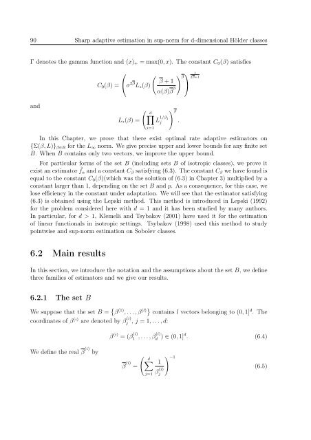
90 Sharp adaptive estimation in sup-norm for d-dimensional Hölder classesΓ denotes the gamma function and (x) + = max(0, x). The constant C 0 (β) satisfiesand⎛C 0 (β) = ⎝σ 2β L ∗ (β)L ∗ (β) =(( d∏i=1) ⎞ ββ + 1⎠α(β)β 3L 1/β jjIn this Chapter, we prove that there exist optimal rate adaptive estimators on{Σ(β, L)} β∈B for the L ∞ norm. We give precise upper and lower bounds for any finite setB. When B contains only two vectors, we improve the upper bound.For particular forms of the set B (including sets B of isotropic classes), we prove itexist an estimator ˜f n and a constant C β satisfying (6.3). The constant C β we have found isequal to the constant C 0 (β)(which was the solution of (6.3) in Chapter 3) multiplied by aconstant larger than 1, depending on the set B and p. As a consequence, for this case, welose efficiency in the constant under adaptation. We will see that the estimator satisfying(6.3) is obtained using the Lepski method. This method is introduced in Lepski (1992)for the problem considered here with d = 1 and it has been studied by many authors.In particular, for d > 1, Klemelä and Tsybakov (2001) have used it for the estimationof linear functionals in isotropic settings. Tsybakov (1998) used this method to studypointwise and sup-norm estimation on Sobolev classes.) β.12β+16.2 Main resultsIn this section, we introduce the notation and the assumptions about the set B, we definethree families of estimators and we give our results.6.2.1 The set BWe suppose that the set B = { β (1) , . . . , β (l)} contains l vectors belonging to (0, 1] d . Thecoordinates of β (i) are denoted by β (i)j , j = 1, . . . , d:β (i) = (β (i)1 , . . . , β (i)d ) ∈ (0, 1]d . (6.4)We define the real β (i) byβ (i) =( d∑j=11β (i)j) −1(6.5)
Page 1:
THÈSE DE DOCTORAT DE L’UNIVERSIT
Page 4 and 5:
Table des matières 1Table des mati
Page 6 and 7:
Table des matières 3.2 Un théorè
Page 8 and 9:
1.1. Objet de la thèse 5blanc gaus
Page 10 and 11:
1.1. Objet de la thèse 7calculées
Page 12 and 13:
1.1. Objet de la thèse 9Un troisi
Page 14 and 15:
1.2. Principaux résultats 11où β
Page 16 and 17:
1.2. Principaux résultats 13le Cha
Page 18 and 19:
1.2. Principaux résultats 15où K
Page 20 and 21:
1.2. Principaux résultats 17de fon
Page 22 and 23:
1.2. Principaux résultats 19L > 0
Page 24 and 25:
Chapitre 2Asymptotically exact esti
Page 26 and 27:
2.2. The main result and the estima
Page 28 and 29:
2.2. The main result and the estima
Page 30 and 31:
2.3. Proofs 27We study the stochast
Page 32 and 33:
2.3. Proofs 29[for ε introduced in
Page 34 and 35:
2.3. Proofs 31where P θ,X is the d
Page 36 and 37:
2.3. Proofs 33as n → ∞ and usin
Page 38 and 39:
2.3. Proofs 35Thus some algebra and
Page 40 and 41:
2.3. Proofs 37Such choice of n is p
Page 42 and 43: 2.4. Appendix of Chapter 2 39• Fi
Page 44 and 45: 3.1. Introduction 41where ψ n = (
Page 46 and 47: 3.2. The estimator and main result
Page 48 and 49: 3.3. Upper bound 45Proof. The stoch
Page 50 and 51: 3.4. Lower bound 473.4 Lower boundB
Page 52 and 53: 3.4. Lower bound 49With these preli
Page 54 and 55: 3.5. Appendix of Chapter 3 51• If
Page 56 and 57: 3.5. Appendix of Chapter 3 53where
Page 58 and 59: Chapitre 4Asymptotically exact mini
Page 60 and 61: 4.2. Main result 57with ˜β define
Page 62 and 63: 4.2. Main result 59(cf. Chapter 5 f
Page 64 and 65: 4.3. Upper bound 61Then we have( )
Page 66 and 67: 4.3. Upper bound 63where N Bj (u) i
Page 68 and 69: 4.4. Lower bound 65is a Gaussian ra
Page 70 and 71: 5.1. Cadre général de l’optimal
Page 72 and 73: 5.2. Application au problème d’a
Page 84 and 85: 5.3. Lien entre l’optimal recover
Page 90 and 91: 5.4. Etudes des constantes 87sente
Page 94 and 95: 6.2. Main results 91and we denote b
Page 96 and 97: 6.2. Main results 936.2.4 Exact asy
Page 98 and 99: 6.2. Main results 952. These result
Page 100 and 101: 6.3. Some preliminary results 97Pro
Page 102 and 103: 6.4. Proof of Theorem 6.1 99Let 0 <
Page 104 and 105: 6.4. Proof of Theorem 6.1 101where
Page 106 and 107: 6.5. Proof of Theorem 6.2 103withA
Page 108 and 109: 6.5. Proof of Theorem 6.2 105The qu
Page 110 and 111: 6.6. Proof of Theorem 6.3 107andwhe
Page 112 and 113: 6.6. Proof of Theorem 6.3 109By Pro
Page 114 and 115: 6.7. Proof of Theorem 6.4 111The pr
Page 116 and 117: 6.8. Proofs of the lemmas and propo
Page 122 and 123: 119Annexe.1 Résultats sur les proc
Page 124 and 125: Bibliographie 121BibliographieAdler
Page 126 and 127: Bibliographie 123Fuller, A. T. (196
Page 128 and 129: Bibliographie 125Micchelli, C. A. a
show all

THÈSE DE DOCTORAT DE L'UNIVERSITÉ PARIS 6 Spécialité ...

Create successful ePaper yourself

Delete template?

Save as template?