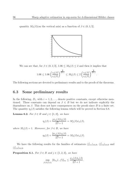
6.2. Main results 952. These results can be generalized to others models such regression with regular design.This can be done by following the same proofs with minor modifications.3. In this chapter, we have considered a finite set B such that its cardinality, card(B),does not depend on n. We could have considered a set B such that card(B) growsas n → ∞ and there exists M > 0 such that, for all β ∈ B, β > M. In Theorems6.2 and 6.4, following the same proofs, it is possible to have the same results1taking B such card(B) ≤ (log n)2(2βmax+1)(The last condition is necessary to havelim n→∞ R 1 (β) = 0 in Section 6.5 and the relation (6.49)). A weaker condition ispossible on B. If, for j ∈ {1, 2, 3}, we replace c j (β) by c j (β) + 1 in η log log n j(β), theresults of Theorem 6.2, Theorem 6.3 and Theorem 6.4 can be obtained for B suchthat card(B) ≤ (log n) a with a > 0.4. For d = 1, in the Lepski method, for a given family of estimators ( ˆf β ) β∈B , wechoose ˆβ, the largest β ∈ B ⊂ R + such that ‖ ˆf β − ˆf γ ‖ ∞ ≤ cψ n (γ) for all γ ≤ β,with a constant c > 0. This choice is based on the fact that, if f ∈ Σ(β v , L) andγ ≤ β ≤ β v , the bias of ˆf β − ˆf γ is upper-bounded by a term of order ψ n (γ). Thisproperty is still valid for anisotropic settings when B satisfies Condition (P ), but itdoes not work for general anisotropic settings. Indeed, for anisotropic settings, wedo not have such a property on the bias of ˆf β − ˆf γ and this bias can be very large.Kerkyacharian et al. (2001) give a new criteria which permits to obtain results inanisotropic Besov classes. Rather than comparing ˆf β to ˆf γ for γ ≤ β, they compare,for γ ≤ β, ˆf γ to a kernel estimator ˆf βγ with bandwidth (h 1 (β, γ), . . . , h d (β, γ)) whereh i (β, γ) = max(h i (β), h i (γ)) and (h 1 (β), . . . , h d (β)), respectively (h 1 (γ), . . . , h d (γ)),is the bandwidth of ˆfβ , respectively ˆf γ . This comparison permits to have a newcriteria for selecting ˆβ. In Theorem 6.3 and Theorem 6.4, we use another estimatorˆf β∗γ,j to do this kind of comparison. The different choice of ˆf β∗γ,j is motivated byour goal to have better constants.5. Our results are adaptation with respect to β and we suppose that L is fixedand known. To use our method of estimation, the statistician need to knowL. Here we suppose the statistician does not know L. We suppose that βbelongs to B and L ∈ {L (1) , . . . , L (l) } ⊂]0, +∞[ d . We note for j = 1, . . . , l,L (j) = (L (j)1 , . . . , L (j)d). Our method can be applied to select β ∈ B with˜L = (max j=1,...,d L (j)1 , . . . , max j=1,...,d L (j)d ).6. Theorem 6.2 gives a result of exact estimation. In Theorem 6.3 and in Theorem 6.4in the case f ∈ Σ(γ, L), the difference between the lower bound and the upper boundis the factor (M 2 (β)) p and (M 3 (γ)) p respectively. The following plot represents the
96 Sharp adaptive estimation in sup-norm for d-dimensional Hölder classesquantity M 3 (β)(on the vertical axis) as a function of β ∈ (0, 1/2].2.01.91.81.71.61.51.41.31.21.11.00.00 0.05 0.10 0.15 0.20 0.25 0.30 0.35 0.40 0.45 0.50We can see that, for β ∈ (0, 1/2], 1.06 ≤ M 3 (β) ≤ 2 and then it implies that1.06 ≤ 1.06( ) βc2 (β)c 1 (β)2β+1≤ M2 (β) ≤ 2(c2 (β)c 1 (β)) β2β+1.The following sections are devoted to preliminary results and to the proofs of the theorems.6.3 Some preliminary resultsIn the following, D i , with i = 1, 2, . . ., denote positive constants, except otherwise mentioned.These constants can depend on β ∈ B but we do not indicate explicitly thedependence on β. This does not have consequences on the proofs since B is a finite set.The quantity η j (β) satisfies the following lemma which will be proved in Section 6.8.Lemma 6.2. For β ∈ B and j ∈ {1, 2}, we haveη j (β) + jψ n(β)λ j (β)2β + 1= M j (β)ψ n (β),where M 1 (β) = 1. Moreover, for β ∈ B, we haveη 3 (β) + 2ψ n(β)λ 3 (β)2β + 1= M 3 (β)ψ n (β).We have the following results for the families of estimators ( ˆf β,1 ) β∈B , ( ˆf β,2 ) β∈B and( ˆf β,3 ) β∈B .Proposition 6.1. For β ∈ B and j ∈ {1, 2, 3}, we havesupf∈Σ(β,L)‖b β,j (·, f)‖ ∞ ≤ ψ n(β)λ j (β).2β + 1