Electronic Devices and Amplifier Circuits

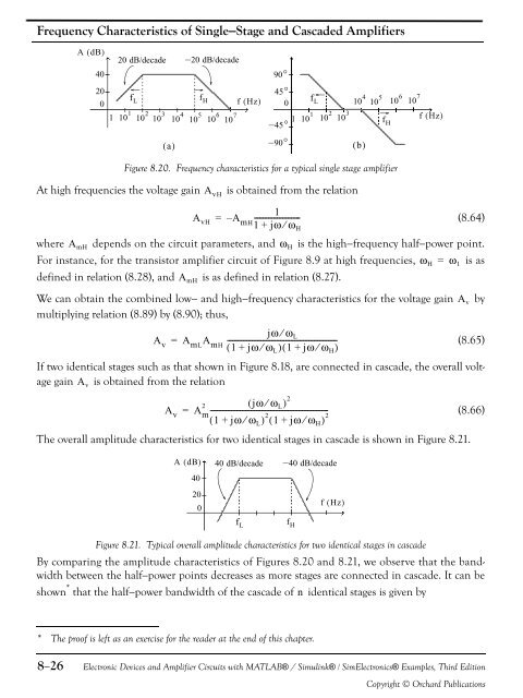
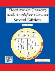
Frequency Characteristics of Single−Stage and Cascaded AmplifiersA ( dB)40200120 dB/decade –20 dB/decadef Lf Hf ( Hz)10 1 10 2 10 3 10 4 10 5 10 6 10 790°45°01–45°( a) –90°( b)f L10 4 10 5 10 6 10 710 1 10 2 10 3 f ( Hz)f HFigure 8.20. Frequency characteristics for a typical single stage amplifierAt high frequencies the voltage gainA vHis obtained from the relation1A vH= – A mH-------------------------(8.64)1+jω⁄ω Hwhere A mH depends on the circuit parameters, and ω H is the high−frequency half−power point.For instance, for the transistor amplifier circuit of Figure 8.9 at high frequencies, ω H = ω 1 is asdefined in relation (8.28), and is as defined in relation (8.27).A mHWe can obtain the combined low− and high−frequency characteristics for the voltage gain A v bymultiplying relation (8.89) by (8.90); thus,jω ⁄ ωA v = A mLA mH--------------------------------------------------------------L(8.65)( 1+jω⁄ω L )( 1 + jω ⁄ ω H )If two identical stages such as that shown in Figure 8.18, are connected in cascade, the overall voltagegain A v is obtained from the relation2 ( jω⁄ωA v A L ) 2= m------------------------------------------------------------------(8.66)( 1 + jω⁄ω L ) 2 ( 1+jω ⁄ ω H ) 2The overall amplitude characteristics for two identical stages in cascade is shown in Figure 8.21.A ( dB) 40 dB/decade – 40 dB/decade40200f ( Hz)f Lf HFigure 8.21. Typical overall amplitude characteristics for two identical stages in cascadeBy comparing the amplitude characteristics of Figures 8.20 and 8.21, we observe that the bandwidthbetween the half−power points decreases as more stages are connected in cascade. It can beshown * that the half−power bandwidth of the cascade of n identical stages is given by* The proof is left as an exercise for the reader at the end of this chapter.8−26Electronic Devices and Amplifier Circuits with MATLAB® / Simulink® / SimElectronics® Examples, Third EditionCopyright © Orchard Publications