Electronic Devices and Amplifier Circuits

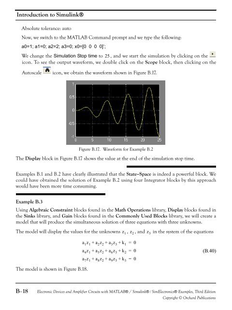
Introduction to Simulink®Absolute tolerance: autoNow, we switch to the MATLAB Command prompt and we type the following:a0=1; a1=0; a2=2; a3=0; x0=[0 0 0 0]’;We change the Simulation Stop time to 25 , and we start the simulation by clicking on theicon. To see the output waveform, we double click on the Scope block, then clicking on theAutoscaleicon, we obtain the waveform shown in Figure B.17.Figure B.17. Waveform for Example B.2The Display block in Figure B.17 shows the value at the end of the simulation stop time.Examples B.1 and B.2 have clearly illustrated that the State−Space is indeed a powerful block. Wecould have obtained the solution of Example B.2 using four Integrator blocks by this approachwould have been more time consuming.Example B.3Using Algebraic Constraint blocks found in the Math Operations library, Display blocks found inthe Sinks library, and Gain blocks found in the Commonly Used Blocks library, we will create amodel that will produce the simultaneous solution of three equations with three unknowns.The model will display the values for the unknowns z 1 , z 2 , and z 3 in the system of the equationsa 1 z 1 + a 2 z 2 + a 3 z 3 + k 1 = 0a 4 z 1 + a 5 z 2 + a 6 z 3 + k 2 = 0a 7 z 1 + a 8 z 2 + a 9 z 3 + k 3 = 0(B.40)The model is shown in Figure B.18.B−18Electronic Devices and Amplifier Circuits with MATLAB® / Simulink® / SimElectronics® Examples, Third EditionCopyright © Orchard Publications