Electronic Devices and Amplifier Circuits

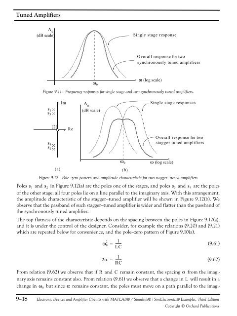
Tuned AmplifiersA c(dB scale)Single stage responseOverall response for twosynchronously tuned amplifiersω 0ω (log scale)Figure 9.11. Frequency responses for single stage and two synchronously tuned amplifiers.s 1s 3ImA c(dB scale)Single stage responsess 4s 2( 2)ReOverall response for twostagger tuned amplifiersω (log scale)Figure 9.12. Pole−zero pattern and amplitude characteristic for two stagger−tuned amplifiersPoles s 1 and s 2 in Figure 9.12(a) are the poles one of the stages, and poles s 3 and s 4 are the polesof the other stage; all four poles lie on a line parallel to the imaginary axis. With this arrangement,the amplitude characteristic of the stagger−tuned amplifier will be shown in Figure 9.12(b). Weobserve that the passband of such stagger−tuned amplifier is wider and flatter than the passband ofthe synchronously tuned amplifier.The top flatness of the characteristic depends on the spacing between the poles in Figure 9.12(a),and it is under the control of the designer. Consider, for example the relations (9.20) and (9.21)which are repeated below for convenience, and the pole−zero pattern of Figure 9.10(a).(9.61)12α = -------(9.62)RCFrom relation (9.62) we observe that if R and C remain constant, the spacing α from the imaginaryaxis remains constant also. From relation (9.61) we observe that a change in L will result in achange in but since α remains constant, the poles must move on a path parallel to the imagi-ω 0ω 0( a) ( b)2 1ω 0 = -------LC9−18Electronic Devices and Amplifier Circuits with MATLAB® / Simulink® / SimElectronics® Examples, Third EditionCopyright © Orchard Publications