Electronic Devices and Amplifier Circuits

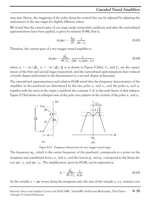
Cascaded Tuned Amplifiersnary axis. Hence, the staggering of the poles along the vertical line can be adjusted by adjusting theinductances in the two stages for slightly different values.We found that the current gain of one stage under sinusoidal conditions and after the narrowbandapproximations have been applied, is given by relation (9.48), that is,Ajω ( )=g------ m 1– ⋅ ---------------2C jω – s 1(9.63)Therefore, the current gain of a two stagger−tuned amplifier isAjω ( )=2g m 1--------------- ⋅ ------------------------------------------4C 1 C 2 ( jω – s 1 )( jω – s 3 )(9.64)where s 1 = – α + jβ 1 , s 3 = – α + jβ 3 , β is as shown in Figure 9.10(a), C 1 and C 2 are the capacitancesof the first and second stages respectively, and the narrowband approximations have reduceda fourth−degree polynomial in the denominator to a second−degree polynomial.The narrowband approximations and relation (9.64) reveal that the frequency characteristics of theamplifier in the passband are determined by the two poles s 1 and s 3 , and the poles s 2 and s 4together with the zeros at the origin contribute the constant 1⁄4 in the scale factor of that relation.Figure 9.13(a) shows an enlarged view of the pole−zero pattern in the vicinity of the poles s 1 and s 3 .Im2λ2βs 1ρ 1ρ 3φsjω cλs 3αω c( a) ( b)Figure 9.13. Frequency characteristic for two stagger−tuned stagesThe frequency ω c, which is the center frequency of the passband, corresponds to a point on theimaginary axis equidistant from s s 1 and s 3 , and the vectors ρ 1 and ρ 3 correspond to the linear factorsjω – s 1 and jω – s 3 . The amplification, given by (9.64), can be expressed asωA=2g--------------- m 1⋅ ----------4C 1 C 2 ρ 1 ρ 3(9.65)As the variable s = jω moves along the imaginary axis, the area of the triangle s 1 s s 3 remains con-Electronic Devices and Amplifier Circuits with MATLAB® / Simulink® / SimElectronics® Examples, Third EditionCopyright © Orchard Publications9−19