Wave Propagation in Linear Media | re-examined

ve/c
1
0.8
0.6
0.4
0.2
0
2.5 5 7.5 10 12.5 15 17.5 20 Z0/R
3Wave propagation in electromagnetic transmission lines
ve/c
1
0.8
0.6
0.4
0.2
0
0.2 0.4 0.6 0.8 1 Z0/R
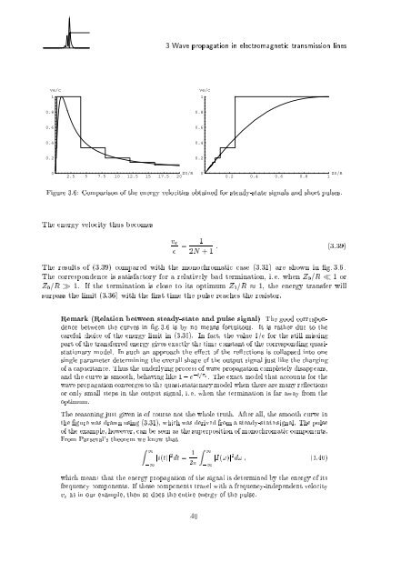
Figure 3.6: Comparison of the energy velocities obtained for steady-state signals and short pulses.
The energy velocity thus becomes
ve
c =
1
: (3.39)
2N +1
The results of (3.39) compared with the monochromatic case (3.31) are shown in g. 3.6 .
The correspondence is satisfactory for a relatively bad termination, i. e. when Z0=R 1 or
Z0=R 1. If the termination is close to its optimum Z0=R 1, the energy transfer will
surpass the limit (3.36) with the rst time the pulse reaches the resistor.
Remark (Relation between steady-state and pulse signal) The good correspondence
between the curves in g. 3.6 is by no means fortuitous. It is rather due to the
careful choice of the energy limit in (3.36). In fact, the value 1=e for the still missing
part of the transferred energy gives exactly the time constant of the corresponding quasistationary
model. In such an approach the e ect of the re ections is collapsed into one
single parameter determining the overall shape of the output signal just like the charging
of a capacitance. Thus the underlying process of wave propagation completely disappears,
and the curve is smooth, behaving like 1,e ,t= e . The exact model that accounts for the
wave propagation converges to the quasi-stationary model when there are many re ections
or only small steps in the output signal, i. e. when the termination is far away from the
optimum.
The reasoning just given is of course not the whole truth. After all, the smooth curve in
the gure was drawn using (3.31), which was derived from a steady-state signal. The pulse
of the example, however, can be seen as the superposition of monochromatic components.
From Parseval's theorem we know that
Z 1
,1
ji(t)j 2 dt = 1
2
Z 1
jI(!)j
,1
2 d! ; (3.40)
which means that the energy propagation of the signal is determined by the energy of its
frequency components. If these components travel with a frequency-independent velocity
ve as in our example, then so does the entire energy of the pulse.
40