Wave Propagation in Linear Media | re-examined

0.8
0.6
0.4
0.2
Y
1
0
3Wave propagation in electromagnetic transmission lines
0 1 2 3 4 5
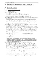
Figure 3.23: Snapshot of the magnetic eld of a TE01 wave. The parameters are = 0:8 and T =4:87 .
propagate without a lower cuto frequency. In fact, this is a surface wave at the interface
between metal and `normal' dielectric, and therefore the geometrical limitations are no
longer relevant. Unfortunately, this mode is associated with a rather high attenuation,
but for small-distance applications, this might be tolerable (see also Paschke [100]).
3.9 A Gaussian pulse in plasma
To round o the results of the previous sections, we now investigate the behaviour of a
Gaussian pulse in a lossless plasma. The model we use is still the transmission line of section
3.5 with the dispersion relation
k(!) = !p
c
s !
!p
2
,1: (3.97)
The boundary condition, i. e. the pulse applied at the interface x = 0, is given by
u(0;t)=U0e , t,t 0 2
Re e j!0t ; (3.98)
where t0 denotes the position of the peak and is the standard deviation of the exponential
distribution. Owing to the linearity of the system, we mayuse the complex notation and take
the real part of the expressions if necessary. The voltage at any point inside the plasma is
then given in the well-known manner as the Fourier integral
u(x; t) =Re
Z 1
,1
A(!) e j(!t,k(!)x) d! : (3.99)
Note that since the pulse has an in nite duration, there is no initial condition to comply
with. Consequently, we cannot apply a trick as in the turn-on case of section 3.7 to make the
evaluation easier, and we have to compute the wave integral directly.
The spectrum A(!) of the initial pulse can easily be calculated, which gives
A(!) = 1
2
Z 1
,1
u(0;t) e ,j!t dt = p e
2 , (!,! 0 )
2
64
2
e ,jt0(!,!0) : (3.100)
X