Wave Propagation in Linear Media | re-examined

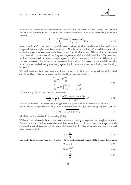
3.7 Turn-on e ects in a lossless plasma
Each of the partial waves that make up the function has a distinct frequency, just like the
steady-state solution (3.69). We can thus immediately write down the transient part of the
current,
It
= , 2 Z 1
sin x cos !( )t
d : (3.74)
I0
0
2 + 0 2
Note that in (3.74) we used a spatial decomposition of the transient solution and not a
temporal one as might have been expected. This is the second signi cant di erence of the
present approach as compared with those known from the literature. All available publications
start from the calculation of the frequency spectrum of the initial conditions. By contrast,
we have determined the wave number spectrum of the boundary conditions. Whether one
chooses one possibility or the other is essentially a matter of opinion. In our special case, the
wave number method was particularly appealing because the transient solution could readily
be found.
We still need the transient solution of the voltage. To that end we recall the di erential
equations that relate current and voltage in the evanescent region,
@U
@x
= ,L0@I
@t
@I !p
= C0
@x
If we insert (3.74) in the rst one, we obtain
Ut
U0L0 = 2 Z 1
0
!
2
, 1 @U
@t :
(3.75)
!( ) cos x sin !( )t
d : (3.76)
2 + 0 2
We recognise that the transient voltage also complies with the boundary conditions (3.72)
and vanishes everywhere for t =0. The dispersion relation !( ) used in (3.74) and (3.76) is
q
!( )= !p 2 +( c) 2 ; (3.77)
which is readily obtained by inverting (3.44).
We havenow collected all components of the wave and can put together the complete solution.
For the numerical evaluation of the wave functions, however, it is advisable to dispense with
the small physical constants and to use scaled variables. To this end we introduce a normalised
integration variable
= c
!p
(3.78)
and scale the space and time coordinates to the wavelength and period of the plasma frequency,
T = !pt (3.79)
X = !px
c
= !0
!p
51
(3.80)
: (3.81)