RF MODULE

More documents

Recommendations

Info

materials usually are in the 10 −22 F/V range. Without this magnification, a detectable 2nd harmonics requires the z direction of the geometry to be much longer, resulting in a large problem. The Gaussian beam is also excited as a pulse in time, using a Gaussian envelope function. This produces a wave package with a Gaussian frequency spectrum. If you have MATLAB, you can calculate the frequency spectrum from a series of time samples with the fast Fourier transform (FFT) using the function fft. Results and Discussion The main purpose of this simulation is to calculate the second harmonic generation when the pulse travels along the 20 µm geometry. So you have to solve for the time it takes for the pulse to enter, pass, and disappear from the volume. The pulse has a characteristic time of 10 fs, and below you can see the pulse after it has traveled 61 fs. Figure 4-11: The pulse after 61 fs. 296 | CHAPTER 4: OPTICS AND PHOTONICS MODELS
After 90 fs the pulse has reached the output boundary (see Figure 4-12). The simulation has to continue for another 30 fs so the pulse completely disappears. Figure 4-12: The pulse after 90 fs. It has now reached the output boundary. The simulation stores the times between 60 fs and 120 fs, which is when the pulse passes the output boundary. The electric field at this boundary has a second harmonic component that can be extracted using FFT. Perform the extraction and transformation at the MATLAB command line. The result appears in Figure 4-13 on page 298. There are two groups of peaks in the figure, where the peaks on the right are mirrors of the ones to the left. This mirror effect is due to the sampling of the harmonic signals, which always creates a mirror spectrum around the sampling frequency. SECOND HARMONIC GENERATION OF A GAUSSIAN BEAM | 297
Page 1 and 2:
COMSOL Multiphysics RF MODULE V ERS
Page 3 and 4:
CONTENTS Chapter 1: Introduction Mo
Page 5 and 6:
Results and Discussion. . . . . . .
Page 7 and 8:
Chapter 4: Optics and Photonics Mod
Page 9 and 10:
1 Introduction The RF Module Model
Page 11 and 12:
highlights. The categories here inc
Page 13 and 14:
TABLE 1-1: RF MODULE MODEL LIBRARY
Page 15 and 16:
2 Tutorial Models This chapter cont
Page 17 and 18:
Results and Discussion Figure 2-1 s
Page 19 and 20:
4 Draw a square with corners at (
Page 21 and 22:
COMPUTING THE SOLUTION Click the So
Page 23 and 24:
Results and Discussion The dipole a
Page 25 and 26:
PHYSICS SETTINGS Variables 1 Choose
Page 27 and 28:
5 Click OK to close the dialog box
Page 29 and 30:
Model Library path: RF_Module/Tutor
Page 31 and 32:
4 From the Solve menu, open the Sol
Page 33 and 34:
them from the eigenvalues. The appl
Page 35 and 36:
5 On the Port page, set the values
Page 37 and 38:
5 On the Port page, enter 36.4 in t
Page 39 and 40:
Waveguide Optimization Introduction
Page 41 and 42:
Results and Discussion Figure 2-3 s
Page 43 and 44:
Modeling Using the Graphical User I
Page 45 and 46:
3 Select Boundary 7 and set the Con
Page 47 and 48:
POSTPROCESSING AND VISUALIZATION Fo
Page 49 and 50:
The solution takes a few minutes to
Page 51 and 52:
Night side Earth surface Ionosphere
Page 53 and 54:
Results and Discussion The model pr
Page 55 and 56:
4 Select both spheres and click the
Page 57 and 58:
RF and Microwave Models In this cha
Page 59 and 60:
measure of the transmittance and re
Page 61 and 62:
y 1 cm is at about 7.5 GHz. At the
Page 63 and 64:
By feeding the circulator at a diff
Page 65 and 66:
Importing the Geometry from a Binar
Page 67 and 68:
MESH GENERATION This model uses the
Page 69 and 70:
It is more instructive to look at t
Page 71 and 72:
Note: When displaying S-Parameter v
Page 73 and 74:
Monoconical RF Antenna Introduction
Page 75 and 76:
50 Ω, to obtain maximum transmiss
Page 77 and 78:
Figure 3-7 shows the antenna radiat
Page 79 and 80:
2 Select the RF Module>Electromagne
Page 81 and 82:
13 Zoom in around (0, 0) using the
Page 83 and 84:
4 In the Contour levels area, click
Page 85 and 86:
2 Clear the Keep current plot check
Page 87 and 88:
6 Click the Solve button on the Mai
Page 89 and 90:
Results and Discussion The figure b
Page 91 and 92:
PHYSICS SETTINGS Point Settings Def
Page 93 and 94:
2 In the x-axis area, select the Ex
Page 95 and 96:
Because the impedance is inversely
Page 97 and 98:
4 From the Space dimension list, se
Page 99 and 100:
2 Select Boundaries 1, 2, 4, and 6.
Page 101 and 102:
4 On the Pointwise Constraints page
Page 103 and 104:
12 Click the Solve button on the Ma
Page 105 and 106:
Module. The electromagnetic cavity
Page 107 and 108:
EIGENFREQUENCY VS. TEMPERATURE By r
Page 109 and 110:
GEOMETRY MODELING 1 Go to the Draw
Page 111 and 112:
3 Set dx, dy, and dz to u, v, and w
Page 113 and 114:
20 Select the Solve using solver se
Page 115 and 116:
Computing the Solution Using a Para
Page 117 and 118:
8 Click Solve. 9 When the parametri
Page 119 and 120:
H-Bend Waveguide with S-parameters
Page 121 and 122:
Model Library path: RF_Module/RF_an
Page 123 and 124:
1 From the Postprocessing menu, cho
Page 125 and 126:
The rectangular port is excited by
Page 127 and 128:
Figure 3-16 shows a single-mode wav
Page 129 and 130:
Figure 3-18: The S 21 parameter (in
Page 131 and 132:
PHYSICS SETTINGS First set up the b
Page 133 and 134:
FREEZING THE BOUNDARY MODE ANALYSIS
Page 135 and 136:
Page 137 and 138:
Microwave Cancer Therapy Introducti
Page 139 and 140:
The model takes advantage of the pr
Page 141 and 142:
DOMAIN AND BOUNDARY EQUATIONS—HEA
Page 143 and 144:
Figure 3-23: The computed microwave
Page 145 and 146:
solutions for both the electromagne
Page 147 and 148:
4 Select Subdomain 1, then enter th
Page 149 and 150:
1 Click the Plot Parameters button
Page 151 and 152:
sar_in_human_head_interp.txt. That
Page 153 and 154:
The bioheat equation produces a sim
Page 155 and 156:
3 Click OK. 4 From the Options menu
Page 157 and 158:
17 In the Work-Plane Settings dialo
Page 159 and 160:
SETTINGS SUBDOMAIN 19 epsilonr_brai
Page 161 and 162:
4 Click the Init tab and type 0 in
Page 163 and 164:
POSTPROCESSING AND VISUALIZATION 1
Page 165 and 166:
The walls of the oven and the waveg
Page 167 and 168:
Figure 3-29: Temperature in the cen
Page 169 and 170:
3 Click the block symbol again and
Page 171 and 172:
2 At the waveguide end, Boundary 23
Page 173 and 174:
4 Click OK to generate the plot bel
Page 175 and 176:
Page 177 and 178:
Because the filter cutoff should be
Page 179 and 180:
the force is applied. Figure 3-32 d
Page 181 and 182:
6 Then the ECAD Import Options dial
Page 183 and 184:
PHYSICS SETTINGS Subdomain Settings
Page 185 and 186:
solver takes more steps than it sto
Page 187 and 188:
3 Select Subdomain 1 and clear the
Page 189 and 190:
Page 191 and 192:
Balanced Patch Antenna for 6 GHz In
Page 193 and 194:
k0 = ω ε0 µ 0 All metallic objec
Page 195 and 196:
divided by the input power. In Figu
Page 197 and 198:
Reference 1. E. Recht and S. Shiran
Page 199 and 200:
10 Select the objects SQ2, CO1, and
Page 201 and 202:
43 Specify two spheres with the fol
Page 203 and 204:
inputs are feeding the antenna, lik
Page 205 and 206:
the width of the PML is equal to λ
Page 207 and 208:
a toggle button that shifts between
Page 209 and 210:
5 Select Coarse solver from the tre
Page 211 and 212:
maxE = max(EdB); minE = min(EdB); E
Page 213 and 214:
exterior of the PML that shows a ve
Page 215 and 216:
13 Choose Extrude from the Draw men
Page 217 and 218:
2 Click the Settings button. 3 In t
Page 219 and 220:
Sea Bed Logging Introduction The Se
Page 221 and 222:
Figure 3-39: Electric field magnitu
Page 223 and 224:
PHYSICS SETTINGS Scalar Variables 1
Page 225 and 226:
Page 227 and 228:
5 Click the General tab. From the P
Page 229 and 230:
Optics and Photonics Models In this
Page 231 and 232:
Model Definition The model is built
Page 233 and 234:
Model Library path: RF_Module/Optic
Page 235 and 236:
PHYSICS SETTINGS Scalar Variables S
Page 237 and 238:
POSTPROCESSING AND VISUALIZATION By
Page 239 and 240:
Model Definition The geometry is a
Page 241 and 242:
2 In the list of application modes,
Page 243 and 244:
Because the refractive index of GaA
Page 245 and 246:
5 Click OK twice to see the followi
Page 247 and 248:
Bandgap Analysis of a Photonic Crys
Page 249 and 250:
a 2 a 3 × b1 = 2π----------------
Page 251 and 252:
The five lowest bands for the (1, 1
Page 253 and 254: Modeling Using the Graphical User I
Page 255 and 256: Subdomain Settings 1 Open the Subdo
Page 257 and 258: 3 Click the Parametric tab. Select
Page 259 and 260: 3 Click OK to see the following plo
Page 261 and 262: fem.appl{1}.prop.analysis = 'harmon
Page 263 and 264: Model Definition The mode analysis
Page 265 and 266: 2 Select the RF Module>Perpendicula
Page 267 and 268: 4 On the Contour page, give Magneti
Page 269 and 270: includes only two independent param
Page 271 and 272: OPTIONS AND SETTINGS 1 Open the Con
Page 273 and 274: The problem becomes well-posed by a
Page 275 and 276: POSTPROCESSING AND VISUALIZATION Th
Page 277 and 278: 7 Click OK. 8 From the Postprocessi
Page 279 and 280: the computed propagation constants
Page 281 and 282: 3 The default eigenmode is the one
Page 283 and 284: Compare these ideal values of the p
Page 285 and 286: Stress-Optical Effects with General
Page 287 and 288: The PDE solved is Navier’s equati
Page 289 and 290: and εx ∂u = ∂x εy ∂v = ∂y
Page 291 and 292: Model Library path: RF_Module/Optic
Page 293 and 294: NAME EXPRESSION DESCRIPTION B2 0.65
Page 295 and 296: 2 In the Subdomain Expressions dial
Page 297 and 298: 4 Initialize the mesh in this geome
Page 299 and 300: Note: This model includes an extens
Page 301 and 302: 3 Enter 1.46 in the text field Sear
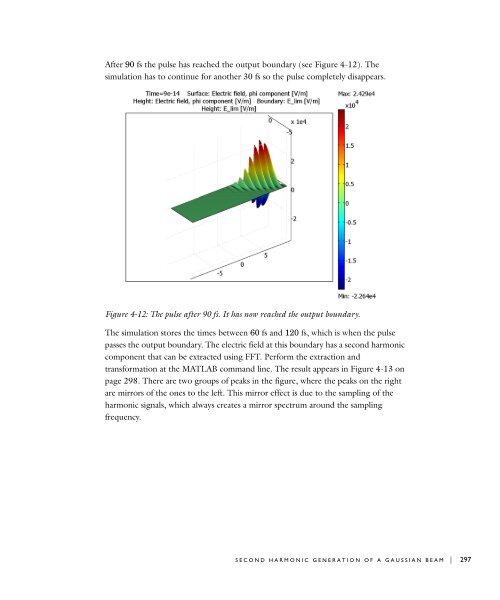
Page 303: In these expressions, w 0 is the mi
Page 307 and 308: 4 Select the RF Module>In-Plane Wav
Page 309 and 310: Boundary Conditions 1 From the Phys
Page 311 and 312: 6 Click the Remesh button; when the
Page 313 and 314: 2 On the General page, make sure th
Page 315 and 316: Propagation of a 3D Gaussian Beam L
Page 317 and 318: Figure 4-15: After 20 fs the pulse
Page 319 and 320: 7 Click the Delete Interior Boundar
Page 321 and 322: Boundary Conditions 1 From the Phys
Page 323 and 324: 5 From the Options menu, select Sup
Page 325 and 326: INDEX 3D electromagnetic waves mode
Page 327 and 328: efractive index 222, 254 resistance
show all

RF MODULE

You also want an ePaper? Increase the reach of your titles

Delete template?

Save as template?