Advanced Building Simulation

102 Hensen
While, in principle, it is possible to combine all matrix equations into one overall
“super-matrix”, this is not done within this software, primarily because of the
advantages that accrue from problem partitioning.
The most immediate advantage is the marked reduction in matrix dimensions and
degree of sparsity—indeed the program never forms two-dimensional arrays for the
above matrices, but instead holds matrix topologies and topographies as sets of vectors.
A second advantage is that it is possible to easily remove partitions as a function
of the problem in hand. For example, when the problem incorporates building-only
considerations, plant-only considerations, plant � flow, and so on. A third advantage
is that different partition solvers can be used which are optimized for the equation
types in question—highly nonlinear, differential and so on.
It is recognized, however, that there often are dominating thermodynamic and/or
hydraulic couplings between the different partitions. If a variable in one partition (say
air temperature of a zone) depends on a variable of state solved within another
partition (say the air flow rate through that zone), it is important to ensure that both
values are matched in order to preserve the thermodynamic integrity of the system.
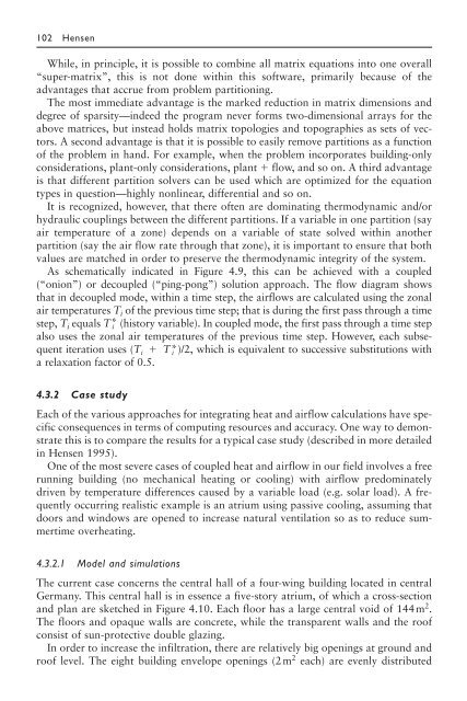
As schematically indicated in Figure 4.9, this can be achieved with a coupled
(“onion”) or decoupled (“ping-pong”) solution approach. The flow diagram shows
that in decoupled mode, within a time step, the airflows are calculated using the zonal
air temperatures Ti of the previous time step; that is during the first pass through a time
step, Ti equals T* i (history variable). In coupled mode, the first pass through a time step
also uses the zonal air temperatures of the previous time step. However, each subsequent
iteration uses (Ti � T*)/2 i , which is equivalent to successive substitutions with
a relaxation factor of 0.5.
4.3.2 Case study
Each of the various approaches for integrating heat and airflow calculations have specific
consequences in terms of computing resources and accuracy. One way to demonstrate
this is to compare the results for a typical case study (described in more detailed
in Hensen 1995).
One of the most severe cases of coupled heat and airflow in our field involves a free
running building (no mechanical heating or cooling) with airflow predominately
driven by temperature differences caused by a variable load (e.g. solar load). A frequently
occurring realistic example is an atrium using passive cooling, assuming that
doors and windows are opened to increase natural ventilation so as to reduce summertime
overheating.
4.3.2.1 Model and simulations
The current case concerns the central hall of a four-wing building located in central
Germany. This central hall is in essence a five-story atrium, of which a cross-section
and plan are sketched in Figure 4.10. Each floor has a large central void of 144m2 .
The floors and opaque walls are concrete, while the transparent walls and the roof
consist of sun-protective double glazing.
In order to increase the infiltration, there are relatively big openings at ground and
roof level. The eight building envelope openings (2m2 each) are evenly distributed