Advanced Building Simulation
Advanced Building Simulation
Advanced Building Simulation

You also want an ePaper? Increase the reach of your titles
YUMPU automatically turns print PDFs into web optimized ePapers that Google loves.
128 Chen and Zhai<br />
(a) 0.6<br />
(b)<br />
U (m/s)<br />
0.4<br />
0.2<br />
0<br />
2<br />
–0.2<br />
–0.4<br />
Exp<br />
0-Equ. model<br />
k-� model<br />
1<br />
Exp<br />
0-Equ. model<br />
k-� model<br />
0<br />
0 0.2 0.4 0.6 0.8 1<br />
0<br />
0 0.2 0.4 0.6 0.8 1<br />
Y/L<br />
(T–Tc )/(Th –Tc )<br />
Figure 5.3 (a) The vertical velocity profile at mid-height and (b) temperature profile in the mid-height<br />
for two-dimensional natural convection case.<br />
than the measurements, although the computed and measured temperature gradients<br />
in the core region are similar. A beginner may not be able to find the reasons for the<br />
discrepancies. With the use of two models, it is possible to find that different models<br />
do produce different results.<br />
Since displacement ventilation consists of natural and forced convection, it is necessary<br />
to simulate a forced convection in order to assess the performance of the<br />
turbulence models. A case proposed by Nielsen (1974) with experimental data is<br />
most appropriate. Due to limited space available, this chapter does not report the<br />
simulation results. In fact, the zero-equation model and the k–� model have performed<br />
similarly for the two-dimensional forced convection case as they did for the<br />
natural convection case reported earlier.<br />
5.3.4 <strong>Simulation</strong> of a three-dimensional case without<br />
internal obstacles<br />
The next step is to simulate a three-dimensional flow. As the problem becomes more<br />
complicated, the experimental data often becomes less detailed and less reliable in<br />
terms of quality. Fortunately, with the experience of the two-dimensional flow simulation,<br />
the three-dimensional case selection is not critical. For example, the experimental<br />
data of mixed convection in a room as shown in Figure 5.4 from Fisher (1995)<br />
seems appropriate for this investigation.<br />
Figure 5.5 presents the measured and calculated air speed contours, which show<br />
the similarity between the measurement and simulation of the primary airflow structures.<br />
The results show that the jet dropped down to the floor of the room after traveling<br />
forward for a certain distance due to the negative buoyancy effect. This<br />
comparison is not as detailed quantitatively as the two-dimensional natural convection<br />
case. However, a CFD user would gain some confidence in his/her results<br />
through this three-dimensional simulation.<br />
X/L<br />
5<br />
4<br />
3