Advanced Building Simulation

224 Malkawi
the effects of the changes and creates new datasets that is directed to the visualizor.
Approximation techniques such as sensitivity analysis can be used to identify crucial
regions in the input parameters or to back-calculate model parameters from the outcome
of physical experiments when the model is complex (reverse sensitivity) (Chen
and Ho 1994). Sensitivity analysis is a study of how the variation in the output of a
model can be apportioned, qualitatively or quantitatively, to different sources of variation
(Saltelli et al. 2000). Its main purpose is to identify the sensitive parameters whose
values cannot be changed without changing the optimal solution (Hillier et al. 1995).
The type of data to be visualized determines the techniques that should be used to
provide the best interaction with it in an immersive environment. To illustrate this
further, fluids, which constitute one component of building simulation, will be used
as an example and discussed in further detail. This will also serve as a background
for the example cases provided later in this chapter.
The typical data types of fluids are scalar quantity, vector quantity, and tensor
quantity. Scalar describes a selected physical quantity that consists of magnitude also
referred to as a tensor of zeroth order. Assigning scalar quantities to space can create
a scalar field, Figure 9.4.
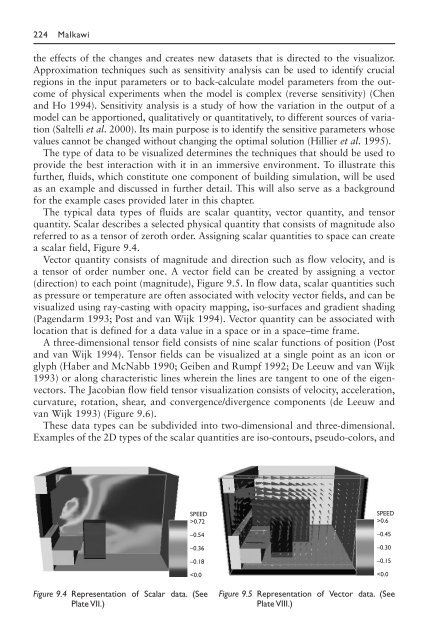
Vector quantity consists of magnitude and direction such as flow velocity, and is
a tensor of order number one. A vector field can be created by assigning a vector
(direction) to each point (magnitude), Figure 9.5. In flow data, scalar quantities such
as pressure or temperature are often associated with velocity vector fields, and can be
visualized using ray-casting with opacity mapping, iso-surfaces and gradient shading
(Pagendarm 1993; Post and van Wijk 1994). Vector quantity can be associated with
location that is defined for a data value in a space or in a space–time frame.
A three-dimensional tensor field consists of nine scalar functions of position (Post
and van Wijk 1994). Tensor fields can be visualized at a single point as an icon or
glyph (Haber and McNabb 1990; Geiben and Rumpf 1992; De Leeuw and van Wijk
1993) or along characteristic lines wherein the lines are tangent to one of the eigenvectors.
The Jacobian flow field tensor visualization consists of velocity, acceleration,
curvature, rotation, shear, and convergence/divergence components (de Leeuw and
van Wijk 1993) (Figure 9.6).
These data types can be subdivided into two-dimensional and three-dimensional.
Examples of the 2D types of the scalar quantities are iso-contours, pseudo-colors, and
SPEED
>0.72
–0.54
–0.36
–0.18
0.6
–0.45
–0.30
–0.15