Back Room Front Room 2

102
where i ∈ [0,w], w is the total number of linear constraints,
j ∈ [1,m1], k ∈ [1,m2], and ars ij , aws
ik , bi are
linear constraint parameters.
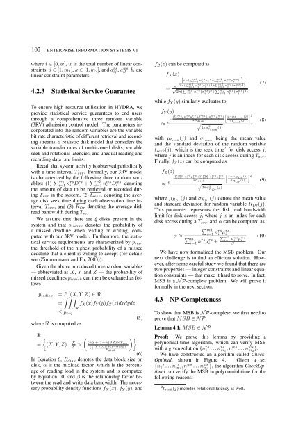
4.2.3 Statistical Service Guarantee
To ensure high resource utilization in HYDRA, we
provide statistical service guarantees to end users
through a comprehensive three random variable
(3RV) admission control model. The parameters incorporated
into the random variables are the variable
bit rate characteristic of different retrieval and recording
streams, a realistic disk model that considers the
variable transfer rates of multi-zoned disks, variable
seek and rotational latencies, and unequal reading and
recording data rate limits.
Recall that system activity is observed periodically
with a time interval Tsvr. Formally, our 3RV model
is characterized by the following three random variables:
(1) �m1 i=1 nrs i Drs i + �m2 i=1 nws i Dws i , denoting
the amount of data to be retrieved or recorded during
Tsvr in the system, (2) tseek, denoting the average
disk seek time during each observation time interval
Tsvr, and (3) RDr denoting the average disk
read bandwidth during Tsvr.
We assume that there are ξ disks present in the
system and that piodisk denotes the probability of
a missed deadline when reading or writing, computed
with our 3RV model. Furthermore, the statistical
service requirements are characterized by preq:
the threshold of the highest probability of a missed
deadline that a client is willing to accept (for details
see (Zimmermann and Fu, 2003)).
Given the above introduced three random variables
— abbreviated as X, Y and Z — the probability of
missed deadlines piodisk can then be evaluated as follows
piodisk = ��� P [(X, Y, Z) ∈ℜ]
= fX(x)fY (y)fZ(z)dxdydz
≤ preq
ℜ
(5)
where ℜ is computed as
ℜ
=
ENTERPRISE INFORMATION SYSTEMS VI
�
(X, Y, Z) | X
ξ >
� (αZ+(1−α)βZ)×Tsvr
Y ×(αZ+(1−α)βZ)
1+ Bdisk ��
(6)
In Equation 6, Bdisk denotes the data block size on
disk, α is the mixload factor, which is the percentage
of reading load in the system and is computed
by Equation 10, and β is the relationship factor between
the read and write data bandwidth. The necessary
probability density functions fX(x), fY (y), and
fZ(z) can be computed as
fX(x)
= e
− [x−(� m1
i=1 nrs
i µrs
i +� m2
i=1 nws
i µws
i )] 2
2×( � m1
i=1 nrs
i (σrs
i )2 + � m2
i=1 nws(σ
i
ws)
i
2 )
√ � m1 2π( i=1 nrs
i (σrs
i )2 + � m2
i=1 nws
i (σws i ) 2 )
while fY (y) similarly evaluates to
fY (y)
≈ e
− (� m1
i=1 nrs
i µrs
i +� m2
i=1 nws
i µws
� �
i
) y−µtseek (j) 2
2Bdisk σtseek (j)
�
2πσ2 t (j)
seek
(7)
(8)
with µtseek (j) and σtseek being the mean value
and the standard deviation of the random variable
tseek(j), which is the seek time2 for disk access j,
where j is an index for each disk access during Tsvr.
Finally, fZ(z) can be computed as
fZ(z)
≈ e
− (� m1
i=1 nrs
i µrs
i +� m2
i=1 nws
i µws
� �
i
) z−µRDr (j) 2
2Bdisk σRDr (j)
�
2πσ2 R (j)
Dr
(9)
where µRDr (j) and σRDr (j) denote the mean value
and standard deviation for random variable RDr(j).
This parameter represents the disk read bandwidth
limit for disk access j, where j is an index for each
disk access during a Tsvr, and α can be computed as
α ≈
�m1 i=1 nrs i µrs i
� m2
i=1 nws
i µws
i
β
� m1
i=1 nrs
i µrs
i +
(10)
We have now formalized the MSB problem. Our
next challenge is to find an efficient solution. However,
after some careful study we found that there are
two properties — integer constraints and linear equation
constraints — that make it hard to solve. In fact,
MSB is a NP-complete problem. We will prove it
formally in the next section.
4.3 NP-Completeness
To show that MSB is NP-complete, we first need to
prove that MSB ∈NP.
Lemma 4.1: MSB ∈NP
Proof: We prove this lemma by providing a
polynomial-time algorithm, which can verify MSB
with a given solution {nrs 1 ...nrs m1 ,nws 1 ...nws m2 }.
We have constructed an algorithm called Check-
Optimal, shown in Figure 4. Given a set
{nrs 1 ...nrs m1 ,nws 1 ...nws m2 }, the algorithm CheckOptimal
can verify the MSB in polynomial-time for the
following reasons:
2 tseek(j) includes rotational latency as well.