Back Room Front Room 2

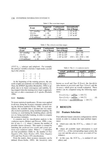
130 ENTERPRISE INFORMATION SYSTEMS VI
Event
Suggested Continuously Intermittently
Range Out of Range Out of Range
BP (mmHg) 90 − 180 ≥ 10 ′ ≥ 10 ′ in 30 ′
O2 (%) ≥ 90 ≥ 10 ′ ≥ 10 ′ in 30 ′
HR (bpm) 60 − 120 ≥ 10 ′ ≥ 10 ′ in 30 ′
UR (ml/hour) ≥ 30 ≥ 1 hour
Critical Suggested Continuously Intermittently Event
Event Range Out of Range Out of Range Anytime
BP (mmHg) 90 − 180 ≥ 60 ′ ≥ 60 ′ in 120 ′ BP < 60
O2 (%) ≥ 90 ≥ 60 ′ ≥ 60 ′ in 120 ′ O2 < 80
HR (bpm) 60 − 120 ≥ 60 ′ ≥ 60 ′ in 120 ′ HR < 30 ∨ HR > 180
UR (ml/hour) ≥ 30 ≥ 2 hours ≤ 10
(SOFAd−1, admtype and admfrom). For example,
the admtype variable is fed into 3 input nodes, according
to the scheme:
1 → −1 −1 1
2 → −1 1 −1
3 → −1 −1 1
At the beginning of the training process, the network
weights are randomly set within the range [-1,1].
Then, the RPROP algorithm (Riedmiller, 1994) is applied,
due to its faster convergence and stability, being
stopped when the training error slope is approaching
zero or after a maximum of E epochs (Prechelt,
1998).
2.2.1 Statistics
To insure statistical significance, 30 runs were applied
in all tests, being the accuracy estimates achieved using
the Holdout method (Flexer, 1996). In each simulation,
the available data is divided into two mutually
exclusive partitions, using stratified sampling: the
training set, used during the modeling phase; and the
test set, being used after training, in order to compute
the accuracy estimates.
A common tool for classification analysis is the
confusion matrix (Kohavi and Provost, 1998), a matrix
of size L × L, where L denotes the number of
possible classes (domain). This matrix is created by
matching the predicted (test result) and actual (patients
real condition) values. When L = 2 and there
are four possibilities (Table 4): the number of True
Negative (TN), False Positive (FP), False Negative
(FN) and True Positive (TP) classifications.
From the matrix, three accuracy measures can be
defined (Essex-Sorlie, 1995): the Sensitivity (also
Table 2: The event time ranges
Table 3: The critical event time ranges
↓ actual \ predicted → negative positive
negative TN FP
positive FN TP
known as recall and Type II Error); the Specificity
(also known as precision and Type I Error); and the
Accuracy, which gives an overall evaluation. These
metrics can be computed using the following equations:
Sensitivity = TP
FN+TP × 100 (%)
Specificity = TN × 100 (%) (4)
Accuracy =
3 RESULTS
Table 4: The 2 × 2 confusion matrix
TN+FP
TN+TP
TN+FP+FN+TP
3.1 Feature Selection
× 100 (%)
Four different feature selection configurations will be
tested, in order to evaluate the input attribute importance:
A - which uses only the SOFAd−1 values (1 variable).
B - where all available input information is used
(SOFAd−1 of the corresponding organ system, the
case mix and the adverse events, in a total of 9 attributes);
C - in this case, the SOFAd−1 is omitted (8 variables);
and