Back Room Front Room 2

(k�
1) (k) (k�1)
(k)
p � w � w
(k)
� g
p G v
u � T �
p v T (k)
v G v
and T represents transpose of a matrix. The problem
with this approach is the requirement of computation
and storage of the approximate Hessian matrix for
every iteration. The One-Step-Secant (OSS) is an
approach to bridge the gap between the conjugate
gradient algorithm and the quasi-Newton (secant)
approach. The OSS approach doesn’t store the
complete Hessian matrix; it assumes that at each
iteration the previous Hessian was the identity
matrix. This also has the advantage that the new
search direction can be calculated without
computing a matrix inverse (Bishop, 1995).
4.4 Support Vector Machines (SVM)
The SVM approach transforms data into a feature
space F that usually has a huge dimension. It is
interesting to note that SVM generalization depends
on the geometrical characteristics of the training
data, not on the dimensions of the input space
(Bishop, 1995; Joachims, 1998). Training a support
vector machine (SVM) leads to a quadratic
optimization problem with bound constraints and
one linear equality constraint. Vapnik (Vladimir,
1995) shows how training a SVM for the pattern
recognition problem leads to the following quadratic
optimization problem (Joachims, 2000):
Minimize:
l
l l
1
W ( � ) � ��
� i � � � yi
y j�
i�
j k(
xi
, x j ) (1)
2
i�1
i�1
j�1
l
Subject to � yi�
i
i�1
�i
: 0 � � i � C
(2)
where l is the number of training examples � is a
vector of l variables and each component
�i corresponds to a training example (xi, yi). The
solution of (1) is the vector *
� for which (1) is
minimized and (2) is fulfilled.
5 EXPERIMENT SETUP
INTRUSION DETECTION SYSTEMS USING ADAPTIVE REGRESSION SPLINES
, v � g
In our experiments, we perform 5-class
classification. The (training and testing) data set
contains 11982 randomly generated points from the
data set representing the five classes, with the
number of data from each class proportional to its
size, except that the smallest classes are completely
,
included. The normal data belongs to class1, probe
belongs to class 2, denial of service belongs to class
3, user to super user belongs to class 4, remote to
local belongs to class 5. A different randomly
selected set of 6890 points of the total data set
(11982) is used for testing MARS, SVMs and
ANNs. Overall accuracy of the classifiers is given in
Tables 1-4. Class specific classification of the
classifiers is given in Table 5.
5.1 MARS
We used 5 basis functions and selected a setting of
minimum observation between knots as 10. The
MARS training mode is being set to the lowest level
to gain higher accuracy rates. Five MARS models
are employed to perform five class classifications
(normal, probe, denial of service, user to root and
remote to local). We partition the data into the two
classes of “Normal” and “Rest” (Probe, DoS, U2Su,
R2L) patterns, where the Rest is the collection of
four classes of attack instances in the data set. The
objective is to separate normal and attack patterns.
We repeat this process for all classes. Table 1
summarizes the test results of the experiments.
5.2 Neural Network
The same data set described in section 2 is being
used for training and testing different neural network
algorithms. The set of 5092 training data is divided
in to five classes: normal, probe, denial of service
attacks, user to super user and remote to local
attacks. Where the attack is a collection of 22
different types of instances that belong to the four
classes described in section 2, and the other is the
normal data. In our study we used two hidden layers
with 20 and 30 neurons each and the networks were
trained using training functions described in Table 2.
The network was set to train until the desired mean
square error of 0.001 was met. As multi-layer feed
forward networks are capable of multi-class
classifications, we partition the data into 5 classes
(Normal, Probe, Denial of Service, and User to Root
and Remote to Local).
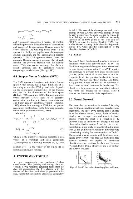
Figure 2: MARS data estimation using splines and knots
215