Back Room Front Room 2

110
ENTERPRISE INFORMATION SYSTEMS VI
This paper is organized as follows. Section 2 discusses
the basic concepts of decision tables. Section
3 then elaborates on how decision diagrams may provide
an alternative, more concise view of the extracted
patterns. Empirical results are presented in section 4.
Section 5 concludes the paper.
2 DECISION TABLES
Decision tables (DTs) are a tabular representation
used to describe and analyze decision situations (e.g.
credit-risk evaluation), where the state of a number of
conditions jointly determines the execution of a set
of actions. A DT consists of four quadrants, separated
by double-lines, both horizontally and vertically.
The horizontal line divides the table into a
condition part (above) and an action part (below).
The vertical line separates subjects (left) from entries
(right). The condition subjects are the criteria that are
relevant to the decision-making process. They represent
the attributes of the rule antecedents about which
information is needed to classify a given applicant as
good or bad. The action subjects describe the possible
outcomes of the decision-making process (i.e.,
the classes of the classification problem: applicant =
good or bad). Each condition entry describes a relevant
subset of values (called a state) for a given condition
subject (attribute), or contains a dash symbol
(‘-’) if its value is irrelevant within the context of that
column (‘don’t care’ entry). Subsequently, every action
entry holds a value assigned to the corresponding
action subject (class). True, false and unknown action
values are typically abbreviated by ‘×’, ‘-’, and ‘.’, respectively.
Every column in the entry part of the DT
thus comprises a classification rule, indicating what
action(s) apply to a certain combination of condition
states. E.g., in Figure 1 (b), the final column tells us
to classify the applicant as good if owns property =
no, and savings amount = high.
If each column only contains simple states (no contracted
or don’t care entries), the table is called an
expanded DT, whereas otherwise the table is called
a contracted DT. Table contraction can be achieved
by combining logically adjacent (groups of) columns
that lead to the same action configuration. For ease of
legibility, we will allow only contractions that maintain
a lexicographical column ordering, i.e., in which
the entries at lower rows alternate before the entries
above them; see Figure 1 (Figure 2) for an example of
an (un)ordered DT, respectively. As a result of this ordering
restriction, a decision tree structure emerges in
the condition entry part of the DT, which lends itself
very well to a top-down evaluation procedure: starting
at the first row, and then working one’s way down the
table by choosing from the relevant condition states,
one safely arrives at the prescribed action (class) for a
given case. The number of columns in the contracted
table can be further minimized by changing the order
of the condition rows. It is obvious that a DT with a
minimal number of columns is to be preferred since
it provides a more parsimonious and comprehensible
representation of the extracted knowledge than an expanded
DT (see Figure 1).
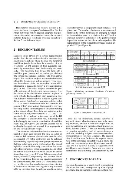
1. Owns property? yes no
2. Years client ≤ 3 >3 ≤ 3 >3
3. Savings amount low high low high low high low high
1. Applicant=good - × × × - × - ×
2. Applicant=bad × - - - × - × -
(a) Expanded DT
1. Owns property? yes no
2. Years client ≤ 3 >3 -
3. Savings amount low high - low high
1. Applicant=good - × × - ×
2. Applicant=bad × - - × -
(b) Contracted DT
1. Savings amount low high
2. Owns property? yes no -
3. Years client ≤ 3 >3 - -
1. Applicant=good - × - ×
2. Applicant=bad × - × -
(c) Minimum-size contracted DT
Figure 1: Minimizing the number of columns of a lexicographically
ordered DT
1. Savings amount high - low low
2. Owns property? - yes no -
3. Years client - >3 - ≤ 3
1. Applicant=good × × - -
2. Applicant=bad - - × ×
Figure 2: Example of an unordered DT
Note that we deliberately restrict ourselves to
single-hit tables, wherein columns have to be mutually
exclusive, because of their advantages with respect
to verification and validation (Vanthienen et al.,
1998). It is this type of DT that can be easily checked
for potential anomalies, such as inconsistencies (a
particular case being assigned to more than one class)
or incompleteness (no class assigned). The decision
table formalism thus facilitates the expert’s assessment
of the knowledge extracted by e.g. a neural network
rule extraction algorithm. What’s more, consulting
a DT in a top-down manner, as suggested above,
should prove more intuitive, faster, and less prone to
human error, than evaluating a set of rules one by one.
3 DECISION DIAGRAMS
Decision diagrams are a graph-based representation
of discrete functions, accompanied by a set of graph
algorithms that implement operations on these func-