Journal of Mechanics of Materials and Structures vol. 5 (2010 ... - MSP

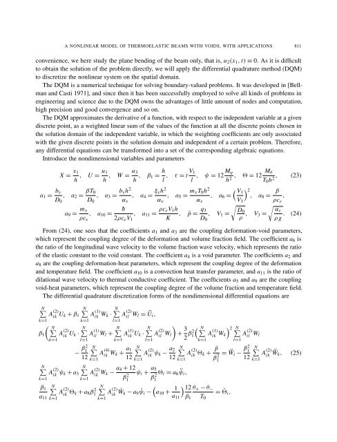
A NONLINEAR MODEL OF THERMOELASTIC BEAMS WITH VOIDS, WITH APPLICATIONS 811
convenience, we here study the plane bending of the beam only, that is, u2(x1, t) ≡ 0. As it is difficult
to obtain the solution of the problem directly, we will apply the differential quadrature method (DQM)
to discretize the nonlinear system on the spatial domain.
The DQM is a numerical technique for solving boundary-valued problems. It was developed in [Bellman
and Casti 1971], and since then it has been successfully employed to solve all kinds of problems in
engineering and science due to the DQM owns the advantages of little amount of nodes and computation,
high precision and good convergence and so on.
The DQM approximates the derivative of a function, with respect to the independent variable at a given
discrete point, as a weighted linear sum of the values of the function at all the discrete points chosen in
the solution domain of the independent variable, in which the weighting coefficients are only associated
with the given discrete points in the solution domain and independent of a certain problem. Therefore,
any differential equations can be transformed into a set of the corresponding algebraic equations.
Introduce the nondimensional variables and parameters
a1 = bv
D0
X = x1
h
u1 u3
, U = , W =
h
, a2 = βT0
, a3 =
D0
a9 = mv
, a10 =
ρce
bvh 2
αv
¯h
2ρceV1
h , β1 = h
,
l
V1
τ = t ,
l
Mϕ
ψ = 12 ,
h2 Mθ
� = 12 ,
T0h 2
(23)
,
ξvh 2 mvT0h 2
a4 = , a5 = ,
αv
αv
� �
V1
2
a6 = , a8 =
V3
β
, a11 =
,
ρce
ρceV1h q3
, ¯p = ,
K D0
�
D0
V1 =
ρ , V3
�
αv
= .
ρχ
(24)
From (24), one sees that the coefficients a1 and a3 are the coupling deformation-void parameters,
which represent the coupling degree of the deformation and volume fraction field. The coefficient a6 is
the ratio of the longitudinal wave velocity to the volume fraction wave velocity, which represents the ratio
of the elastic constant to the void constant. The coefficient a4 is a void parameter. The coefficients a2 and
a8 are the coupling deformation-heat parameters, which represent the coupling degree of the deformation
and temperature field. The coefficient a10 is a convection heat transfer parameter, and a11 is the ratio of
dilational wave velocity to thermal conductive coefficient. The coefficients a5 and a9 are the coupling
void-heat parameters, which represent the coupling degree of the volume fraction and temperature field.
The differential quadrature discretization forms of the nondimensional differential equations are
N�
A (2)
k=1
β1
� N�
k=1
N�
l=1
A (1)
ik Wk · N�
ik Uk + β1
k=1
l=1
A (2)
ik Uk · N�
A (1)
il Wl + N�
N�
A (2)
k=1
β1
− β2 1
ik ψk + a3
k=1
N�
a11 k=1
A (2)
ik �k + a8β 2 1
k=1
A (2)
il Wl = Üi,
A (1)
ik Uk · N�
N�
A
12 k=1
(4)
ik Wk + a1
N�
12 k=1
N�
A (2)
ik Wk − a4 + 12
N�
k=1
A (2)
ik
β 2 1
l=1
A (2)
il Wl
�
+ 3
2 β2 � N�
1 A
k=1
(1)
ik Wk
�2 N�
A
l=1
(2)
il Wl
A (2)
ik ψk − a2
12
ψi + a5
β2 1
˙Wk − a9 ˙ψi −
N�
k=1
�i = a6 ¨ψi,
�
a10 + 1
�
12
a11
A (2)
ik �k + ¯p
β 2 1
β1
θ+ − θ−
T0
= ¨Wi − β2 1
12
= ˙�i,
N�
k=1
A (2)
ik
¨Wk,
(25)