Journal of Mechanics of Materials and Structures vol. 5 (2010 ... - MSP

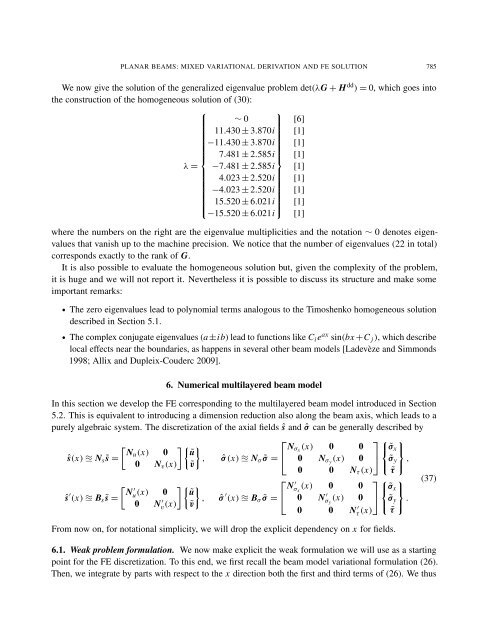
PLANAR BEAMS: MIXED VARIATIONAL DERIVATION AND FE SOLUTION 785
We now give the solution of the generalized eigenvalue problem det(λG + Hdd ) = 0, which goes into
the construction of the homogeneous solution of (30):
⎧
⎫
∼ 0 [6]
11.430 ± 3.870i [1]
−11.430 ± 3.870i [1]
⎪⎨ 7.481 ± 2.585i ⎪⎬ [1]
λ = −7.481 ± 2.585i [1]
4.023 ± 2.520i [1]
−4.023 ± 2.520i [1]
⎪⎩
15.520 ± 6.021i
⎪⎭
[1]
−15.520 ± 6.021i [1]
where the numbers on the right are the eigenvalue multiplicities and the notation ∼ 0 denotes eigenvalues
that vanish up to the machine precision. We notice that the number of eigenvalues (22 in total)
corresponds exactly to the rank of G.
It is also possible to evaluate the homogeneous solution but, given the complexity of the problem,
it is huge and we will not report it. Nevertheless it is possible to discuss its structure and make some
important remarks:
• The zero eigenvalues lead to polynomial terms analogous to the Timoshenko homogeneous solution
described in Section 5.1.
• The complex conjugate eigenvalues (a±ib) lead to functions like Cie ax sin(bx +C j), which describe
local effects near the boundaries, as happens in several other beam models [Ladevèze and Simmonds
1998; Allix and Dupleix-Couderc 2009].
6. Numerical multilayered beam model
In this section we develop the FE corresponding to the multilayered beam model introduced in Section
5.2. This is equivalent to introducing a dimension reduction also along the beam axis, which leads to a
purely algebraic system. The discretization of the axial fields ˆs and ˆσ can be generally described by
⎡
⎤ ⎧ ⎫
� � � �
Nσx (x) 0 0 ⎨ ˜σx ⎬
Nu(x) 0 ũ
ˆs(x) ≅ Ns ˜s =
, ˆσ (x) ≅ Nσ ˜σ = ⎣ 0 Nσy (x) 0 ⎦ ˜σy
0 Nv(x) ˜v
⎩ ⎭
0 0 Nτ (x) ˜τ
,
ˆs ′ �
N ′
(x) ≅ Bs ˜s = u (x) 0
0 N ′ v (x)
� � �
ũ
, ˆσ
˜v
′ ⎡
N
(x) ≅ Bσ ˜σ = ⎣
′ σx (x) 0 0
0 N ′ σy (x) 0
0 0 N ′ τ (x)
⎤ ⎧ ⎫
⎨ ˜σx ⎬
⎦ ˜σy
⎩ ⎭
˜τ
.
(37)
From now on, for notational simplicity, we will drop the explicit dependency on x for fields.
6.1. Weak problem formulation. We now make explicit the weak formulation we will use as a starting
point for the FE discretization. To this end, we first recall the beam model variational formulation (26).
Then, we integrate by parts with respect to the x direction both the first and third terms of (26). We thus