Journal of Mechanics of Materials and Structures vol. 5 (2010 ... - MSP

782 FERDINANDO AURICCHIO, GIUSEPPE BALDUZZI AND CARLO LOVADINA
We can compute ˆσ from the second equation and substitute it into the first, obtaining a displacementlike
formulation of the problem:
where
Aˆs ′′ + Bˆs ′ + C ˆs = 0 + suitable boundary conditions, (32)
A = −Gsσ H −1
σ σ Gσ s, B = −Gsσ H −1
σ σ Hσ ′ s + Hsσ ′ H−1 σ σ Gσ s, C = Hsσ ′ H−1 σ σ Hσ ′ s.
Similar considerations apply to problem (23).
5. Examples of beam models
In this section we give two examples of beam models developed using the strategies of Section 4. More
precisely, starting from the HR div-div approach in Equation (30), we derive
• a single layer beam model in which we use a first-order displacement field, thus showing that the
approach under discussion is able to reproduce the classical models; and
• a multilayer beam model, in which we consider also higher-order kinematic and stress fields, thus
illustrating how the approach can produce a refined model with a reasonable solution.
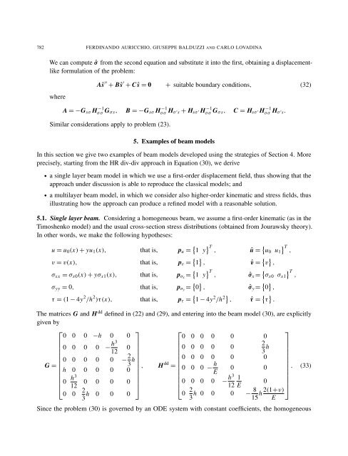
5.1. Single layer beam. Considering a homogeneous beam, we assume a first-order kinematic (as in the
Timoshenko model) and the usual cross-section stress distributions (obtained from Jourawsky theory).
In other words, we make the following hypotheses:
u = u0(x) + yu1(x), that is, pu = � 1 y �T � �T , û = u0 u1 ,
v = v(x), that is, pv = � 1 � , ˆv = � v � ,
σxx = σx0(x) + yσx1(x), that is, pσx = � 1 y �T , ˆσx = � �T σx0 σx1 ,
σyy = 0, that is, pσy = � 0 � , ˆσy = � 0 � ,
τ = (1 − 4y 2 /h 2 )τ(x), that is, pτ = � 1 − 4y 2 /h 2� , ˆτ = � τ � .
The matrices G and Hdd defined in (22) and (29), and entering into the beam model (30), are explicitly
given by
⎡
0 0 0 −h 0 0
⎢
0 0 0 0 −
⎢
G = ⎢
⎣
h3
0
12
0 0 0 0 0 − 2
3 h
h 0 0 0 0 0
0 h3
0 0 0 0
12
0 0 2
⎤
⎥ , H
⎥
⎦
h 0 0 0
3 dd ⎡
0 0 0 0 0 0
⎢
2
0 0 0 0 0
⎢
3
⎢
= ⎢
⎣
h
0 0 0 0 0 0
0 0 0 − h
0 0
E
0 0 0 0 − h3 1
0
12 E
0 2
⎤
⎥ . (33)
⎥
⎦
8 2(1+ν)
h 0 0 0 − h
3 15 E
Since the problem (30) is governed by an ODE system with constant coefficients, the homogeneous