Journal of Mechanics of Materials and Structures vol. 5 (2010 ... - MSP

PLANAR BEAMS: MIXED VARIATIONAL DERIVATION AND FE SOLUTION 787
We remark that this choice of the FE shape functions assures the stability and convergence of the
resulting discrete scheme. We also notice that the stresses are discontinuous across elements along the
x direction, so that it is possible to statically condensate them out at the element level, reducing the
dimension of the global stiffness matrix and improving efficiency.
6.2. Multilayered homogeneous beam. We now consider the same three layer homogeneous beam of
Section 5.2.1. Together with the clamping condition in A0, we assume that l = 10 mm and the beam is
loaded along Al by the quadratic shear stress distribution t|Al = [0, 3/2(1 − 4y2 )] T MPa.
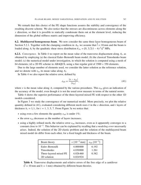
6.2.1. Convergence. In Table 4 we report on the mean value of the transverse displacement along Al, as
obtained by employing (a) the classical Euler–Bernoulli beam model; (b) the classical Timoshenko beam
model; (c) the numerical model under investigation, in which the solution is computed using a mesh of
64 elements; (d) a 2D FE scheme in ABAQUS, using a fine regular grid of 3500 × 350 elements.
Due to the large number of elements used, we consider the latter solution as the reference solution,
and we denote with vex its mean value along Al.
In Table 4 we also report the relative error, defined by
erel =
|v − vex|
, (41)
where v is the mean value along Al computed by the various procedures. This erel gives an indication of
the accuracy of the model, even though it is not the usual error measure in terms of the natural norms.
Table 4 shows the superior performance of the three-layered mixed FE with respect to the other 1D
models considered.
In Figure 3 we study the convergence of our numerical model. More precisely, we plot the relative
quantity defined in (41), evaluated considering different mesh sizes δ in the x direction, and i layers of
thickness hi = 1/i, for i = 1, 3, 5, 7. From Figure 3a we notice that:
|vex|
• using even a few elements the quantity erel is under 1%;
• the error erel decreases as the number of layers increases;
• using a highly refined mesh, the relative error erel increases, even as it apparently converges to a
constant close to 10 −3 . This behavior can be explained by recalling that a modeling error necessarily
arises. Indeed, the solution of the 2D elastic problem and the solution of the multilayered beam
mixed model do differ from each other, for a fixed length and thickness of the beam.
Beam theory v [10 −2 mm] erel [10 −3 ]
Euler–Bernoulli 4.000000 6.192
Timoshenko 4.030000 1.261
Three-layered mixed FE 4.026460 0.382
2D solution 4.024924
Table 4. Transverse displacements and relative errors of the free edge of a cantilever
(l = 10 mm and h = 1 mm) obtained by different beam theories.