Journal of Mechanics of Materials and Structures vol. 5 (2010 ... - MSP

846 ANDREY V. PYATIGORETS, MIHAI O. MARASTEANU, LEV KHAZANOVICH AND HENRYK K. STOLARSKI
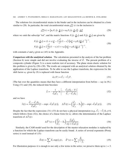
The solutions for circumferential strains in the binder and in the inclusion can be obtained in a form
similar to (28). In particular, the total circumferential strain εinc θθ (r) in the inclusion is
ε inc
θθ (r) = � � � � ��
αi F1 r, Eb + αb F2 r, Eb · �T (29)
� � � �
where we omit the subscript “tot”, and the matrix functions F1 r, Eb and F2 r, Eb are given by
� �
F1 r, Eb = (1 + νi)I − 2 r 2 1
r 2 (1 − ν2 i )� d I + gEi
� � r
F2 r, Eb = 2 2 1
r 2 (1 − νi)(1 + νb) � d I + gEi
with constants d and g given as (A5) in the Appendix.
� �−1�−1, Eb
� �−1�−1, Eb
Comparison with the analytical solution. The calculations presented in the analysis of the bar problem
(Section 6) were simple and did not involve evaluating the inverse of ˜E. The present problem of a
composite cylinder (Figure 3) is a more realistic test of accuracy. The plane strain elastic solution for
this problem is given by (28)–(30). The results are compared with an analytical solution obtained by the
application of the Laplace transform. To be able to use the Laplace transform, the expression for the
shift factor aT given by (9) is replaced with linear function
(30)
âT (T ) = Ĉ1 − Ĉ2T, (31)
(The hat over the quantities means that they have a different interpretation from before — say in (9).)
Using (31) and (10), the reduced time becomes
ˆξ = − 1
�
�
�
ln �
� 1 + Ĉ2(T0
�
− T )
�
�
�
(32)
�
and we have
ˆt(ξ) = Ĉ1 − Ĉ2T0
Ĉ0 Ĉ2
Ĉ0 Ĉ2
Ĉ1 − Ĉ2T0
�
1 − exp(−Ĉ0Ĉ2ξ) � � �
Ĉ1 �1
, � ˆT (ξ) = − T0 − exp(−Ĉ0
Ĉ2
Ĉ2ξ) � . (33)
Despite the fact that the expressions (31)–(33) do not have a physical interpretation (e.g., Ĉ1 − Ĉ2T0 �= 0,
which follows from (32)), the choice of a linear form for âT allows the determination of the Laplace
transform of � ˆT (ξ):
� ˆT ∗ � �
Ĉ1 Ĉ0
(s) = − T0
Ĉ2
Ĉ2
s � s + Ĉ0Ĉ2 �. (34)
Similarly, the CAM model used for the description of the master relaxation modulus is replaced by
a function for which the Laplace transform can be easily found. A series of several exponents (Prony
series) is used instead of (15):
Ê(ξ) = �
Êi exp(ˆγ iξ), Ê ∗ (s) = � Êi
. (35)
s − ˆγ i
i
For illustration purposes it is enough to use only a few terms in the series; we preserve them up to i = 3.
i