Journal of Mechanics of Materials and Structures vol. 5 (2010 ... - MSP

786 FERDINANDO AURICCHIO, GIUSEPPE BALDUZZI AND CARLO LOVADINA
obtain: Find ˆs ∈ ˜W and ˆσ ∈ ˜S such that, for every δˆs ∈ ˜W and for every δ ˆσ ∈ ˜S,
�
δ JHR = (δ ˆs ′T Gsσ ˆσ − δˆs T Hsσ ′ ˆσ + δ ˆσ T Gσ s ˆs ′ − δ ˆσ T Hσ ′ s ˆs − δ ˆσ T Hσ σ ˆσ )dx − δˆs T Tx| x=l = 0, (38)
l
where ˜W := {ˆs ∈ H 1 (l) : ˆs|x=0 = 0} and ˜S := L 2 (l).
Notice that all the derivatives with respect to x are applied to displacement variables, whereas the
derivatives with respect to y (incorporated into the H matrices) are applied to cross-section stress vectors.
The resulting variational formulation has the following features:
• The obtained weak formulation (38) is symmetric.
• y-derivatives applied to stresses and the essential conditions of S dd
t (see Section 3.2.2) most likely
lead to a formulation which accurately solves the equilibrium equation in the y direction, that is, in
the cross-section.
• x derivatives applied to displacements and the essential condition in ˜W most likely lead to a formulation
which accurately solves the compatibility equation along the beam axis.
The FE discretization simply follows from the application of (37) to the variational formulation (38):
�
δ JHR =
l
� T T
δ˜s Bs Gsσ Nσ ˜σ − δ˜s T N T s Hsσ ′ Nσ ˜σ + δ ˜σ T N T σ Gσ s Bs ˜s ′� dx
�
� T T
− δ ˜σ Nσ Hσ
l
′ s Ns ˜s + δ ˜σ T N T σ Hσ σ Nσ ˜σ � dx − δ˜s T N T s Tx| x=l = 0. (39)
Collecting unknown coefficients in a vector and requiring (39) to be satisfied for all possible virtual fields
we obtain �
0
Kσ s
� � � � �
Ksσ ˜s ˜T
= ,
Kσ σ ˜σ 0
(40)
where
Ksσ = K T σ s =
�
(B
l
T s Gsσ Nσ − N T s Hsσ ′ Nσ
�
)dx, Kσ σ = − N
l
T σ Hσ σ Nσ dx, ˜T = N T s Tx| x=l .
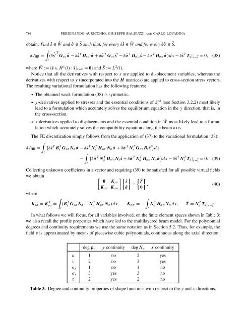
In what follows we will focus, for all variables involved, on the finite element spaces shown in Table 3;
we also recall the profile properties which have led to the multilayered beam model. For the polynomial
degrees and continuity requirements we use the same notation as in Section 5.2. Thus, for example, the
field v is approximated by means of piecewise cubic polynomials, continuous along the axial direction.
deg pγ y continuity deg Nγ x continuity
u 1 no 2 yes
v 2 no 3 yes
σx 1 no 1 no
σy 3 yes 3 no
τ 2 yes 2 no
Table 3. Degree and continuity properties of shape functions with respect to the y and x directions.