Journal of Mechanics of Materials and Structures vol. 5 (2010 ... - MSP

718 BAHATTIN KILIC AND ERDOGAN MADENCI
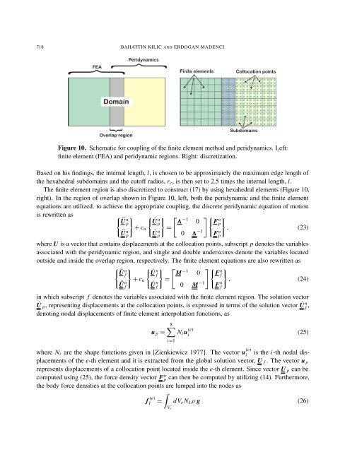
Figure 10. Schematic for coupling of the finite element method and peridynamics. Left:
finite element (FEA) and peridynamic regions. Right: discretization.
Based on his findings, the internal length, l, is chosen to be approximately the maximum edge length of
the hexahedral subdomains and the cutoff radius, rc, is then set to 2.5 times the internal length, l.
The finite element region is also discretized to construct (17) by using hexahedral elements (Figure 10,
right). In the region of overlap shown in Figure 10, left, both the peridynamic and the finite element
equations are utilized. to achieve the appropriate coupling, the discrete peridynamic equation of motion
is rewritten as � � �
Ü n ˙U p
+ cn
n � � −1
p � 0
=
0 � −1
� � �
Fn p
, (23)
Ü n p
˙U n p
where U is a vector that contains displacements at the collocation points, subscript p denotes the variables
associated with the peridynamic region, and single and double underscores denote the variables located
outside and inside the overlap region, respectively. The finite element equations are also rewritten as
� � � n Ü ˙U f
+ cn
n� �
f M−1 0
=
0 M−1 � � � n Ff , (24)
Ü n f
˙U n f
in which subscript f denotes the variables associated with the finite element region. The solution vector
˙U p, representing displacements at the collocation points, is expressed in terms of the solution vector ˙U n f ,
denoting nodal displacements of finite element interpolation functions, as
u p =
8�
i=1
Ni u (e)
i
where Ni are the shape functions given in [Zienkiewicz 1977]. The vector u (e)
i is the i-th nodal displacements
of the e-th element and it is extracted from the global solution vector, U f . The vector u p
represents displacements of a collocation point located inside the e-th element. Since vector U p can be
computed using (25), the force density vector Fn p can then be computed by utilizing (14). Furthermore,
the body force densities at the collocation points are lumped into the nodes as
f (e)
I =
�
Ve
F n p
F n f
(25)
dVe NI ρ g (26)