Journal of Mechanics of Materials and Structures vol. 5 (2010 ... - MSP

PLANAR BEAMS: MIXED VARIATIONAL DERIVATION AND FE SOLUTION 789
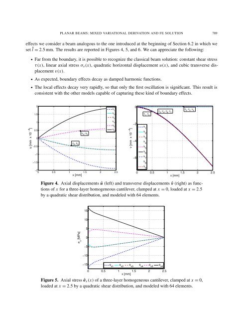
effects we consider a beam analogous to the one introduced at the beginning of Section 6.2 in which we
set l = 2.5 mm. The results are reported in Figures 4, 5, and 6. We can appreciate the following:
u [mm x 10 −4 ]
• Far from the boundary, it is possible to recognize the classical beam solution: constant shear stress
τ(x), linear axial stress σx(x), quadratic horizontal displacement u(x), and cubic transverse displacement
v(x).
• As expected, boundary effects decay as damped harmonic functions.
• The local effects decay very rapidly, so that only the first oscillation is significant. This result is
consistent with the other models capable of capturing these kind of boundary effects.
2
1.5
1
0.5
0
−0.5
−1
−1.5
u 2 , u 3
u 4 , u 5
−2
0 0.5 1 1.5 2 2.5
x [mm]
u 1
u 2
u 3
u 4
u 5
u 6
v [mm x 10 −4 ]
0
−2
−4
−6
v 1 , v 9
v 1
v 2
v 3
v 4
v 5
v 6
v 7
v 8
v 9
v 3 , v 4 , v 6 , v 7
v 2 , v 5 , v 8
0 0.5 1 1.5 2 2.5
x [mm]
Figure 4. Axial displacements û (left) and transverse displacements ˆv (right) as functions
of x for a three-layer homogeneous cantilever, clamped at x = 0, loaded at x = 2.5
by a quadratic shear distribution, and modeled with 64 elements.
σ x [MPa]
15
10
5
0
−5
−10
−15
s x1
s x2
s x3
s x4
s x5
s x6
0 0.5 1 1.5 2 2.5
x [mm]
Figure 5. Axial stress ˆσx(x) of a three-layer homogeneous cantilever, clamped at x = 0,
loaded at x = 2.5 by a quadratic shear distribution, and modeled with 64 elements.