Journal of Mechanics of Materials and Structures vol. 5 (2010 ... - MSP

KIRCHHOFF HYPOTHESIS AND BENDING OF BIMODULAR THIN PLATES 763
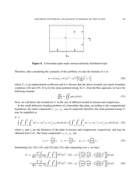
Figure 4. A bimodular plate under normal uniformly distributed loads.
Therefore, after considering the symmetry of this problem, we take the formula of w as
w = C1wm = C1(x 2 − a 2 ) 2�� �
y 2 �
+ 1 , (30)
4b
where C1 is an undetermined coefficient and it is obvious that the above formula can satisfy boundary
conditions (28) and (29). If we let the strain potential energy be U, from the Ritz approach, we have the
following formula:
∂U
∂C1
��
=
qwm dx dy. (31)
Next, we will derive the formula for U in the case of different moduli in tension and compression.
In the small-deflection bending problem of a bimodular thin plate, according to the computational
hypotheses, the strain components εz, γyz, γzx may be neglected; therefore, the strain potential energy U
may be simplified as
U =
1
2
� a � b � t1
(σ
−a −b 0
+
x εx +σ + +
εy+τ y
xy γxy)dx dy dz+ 1
2
� a � b � 0
(σ
−a −b −t2
−
x εx +σ − −
εy+τ y
xy γxy)dx dy dz, (32)
where t1 and t2 are the thickness of the plate in tension and compression, respectively, and may be
obtained from (14). The strain components εx, εy, γxy are
εx = − ∂2w ∂x 2 z, εy = − ∂2w ∂y 2 z, γxy = −2 ∂2w z. (33)
∂x∂y
Substituting (9), (10), (15), and (33) into (32), after integrating over z, we have
E
U =
+ t3 1
6[1 − (µ + ) 2 � a � b �
(∇
] −a −b
2 w) 2 − 2(1 − µ + �
∂2w )
∂x 2
∂2w �
∂2 � ��
w 2
−
dx dy
∂y 2 ∂x∂y
E
+
−t 3 2
6[1 − (µ − ) 2 � a � b �
(∇
]
2 w) 2 − 2(1 − µ − �
∂2w )
∂x 2
∂2w �
∂2 � ��
w 2
−
dx dy. (34)
∂y 2 ∂x∂y
−a
−b