Journal of Mechanics of Materials and Structures vol. 5 (2010 ... - MSP

740 A. H. GANDOMI, A. H. ALAVI, P. ARJMANDI, A. AGHAEIFAR AND R. SEYEDNOUR
x0
+
x1
C D
A
+
x2
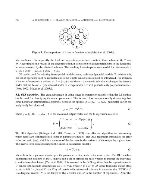
Figure 5. Decomposition of a tree to function terms [Madár et al. 2005a].
also nonlinear. Consequently, the final decomposition procedure results in three subtrees: B, C, and
D. According to the results of the decomposition, it is possible to assign parameters to the functional
terms represented by the obtained subtrees. The resulting linear-in-parameters model for this example is
y : p0 + p1(x2 + x1)/x0 + p2x0 + p3x1.
GP can be used for selecting from special model classes, such as polynomial models. To achieve this,
the set of operators must be restricted and some simple syntactic rules must be introduced. For instance,
if the set of operators is defined as F = {×, +} and there is a syntactic rule that exchanges the internal
nodes that are below ×-type internal nodes to ×-type nodes, GP will generate only polynomial models
[Koza 1992; Madár et al. 2005a].
3.2. OLS algorithm. The great advantage of using linear-in-parameter models is that the LS method
can be used for identifying the model parameters. This is much less computationally demanding than
other nonlinear optimization algorithms, because the optimal p = [p1, . . . , pm]T parameter vector can
analytically be calculated:
p = (U −1 U) T Uy, (1)
where y = (y(1), . . . , y(N))T is the measured output vector and the U regression matrix is
⎛
⎞
U1(x(1)) · · · UM(x(1))
⎜
U = ⎝
.
. ..
⎟
. ⎠ . (2)
U1(x(N)) · · · UM(x(N))
The OLS algorithm [Billings et al. 1988; Chen et al. 1989] is an effective algorithm for determining
which terms are significant in a linear-in-parameters model. The OLS technique introduces the error
reduction ratio (err), which is a measure of the decrease in the variance of the output by a given term.
The matrix form corresponding to the linear-in-parameters model is
+
B
/
x1
x0
y = Up + e, (3)
where U is the regression matrix, p is the parameter vector, and e is the error vector. The OLS method
transforms the columns of the U matrix into a set of orthogonal basis vectors to inspect the individual
contributions of each term [Cao et al. 1999]. It is assumed in the OLS algorithm that the regression matrix
U can be orthogonally decomposed as U = W A, where A is a M by M upper triangular matrix (that
is, Ai j = 0 if i > j) and W is a N by M matrix with orthogonal columns in the sense that W T W = D
is a diagonal matrix (N is the length of the y vector and M is the number of repressors). After this