Journal of Mechanics of Materials and Structures vol. 5 (2010 ... - MSP

812 YING LI AND CHANG-JUN CHENG
( j)
where i ranges from 1 to N, the number of discrete points, and A ik is the weighting coefficient of
the j-th partial derivative of the function with respect to the independent variable X. In this paper, the
polynomial function is adopted as the test function to obtain the weighting coefficient, and the zeros of
the Chebyshev–Lobatto polynomial are adopted as the coordinates of the grid points [Bellman and Casti
1971].
The DQ discretization forms of the nondimensional boundary conditions can be expressed as
N�
k=1
U1 = UN = 0, W1 = WN = 0, �1 = �N = 0,
A (1)
1k ψk =
N�
k=1
A (1)
Nk ψk = 0,
N�
k=1
A (1)
1k Wk =
N�
k=1
A (1)
Nk Wk = 0.
If the initial values of variables are all zero, we have the initial conditions of nondimensional forms
(26)
U(0) = ˙U(0) = W (0) = ˙W (0) = ψ(0) = ˙ψ(0) = �(0) = 0 (27)
Assuming that the temperature distribution is given by θ(x1, x3) = θ0(1/2 + x3/h), we have θ+ = θ0,
θ− = 0.
Hence, the static problem is converted to solving the nonlinear algebraic equations (25) under the
boundary conditions (26); while the dynamical problem is converted to solving the nonlinear ordinary
differential equations (25) under the boundary conditions (26) and initial condition (27). The Newton–
Raphson and Runge–Kutta methods are adopted in the calculation of the static and dynamical problems,
respectively.
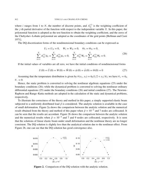
To illustrate the correctness of the theory and method in this paper, a simply supported elastic beam
subjected to a uniformly distributed load ¯p is considered. The analytic solution is available in the case
of small deformation. Figure 2a shows the comparison between the analytic solution and the numerical
result obtained from the theory and method of this paper when ¯p = 10 −5 and 7 nodes are collocated. It
can be seen that the results are accordant. Figure 2b shows the comparison between the analytic solution
and the numerical results when ¯p = 10 −4 and 7 and 9 nodes are collocated, respectively. It is seen
that the solutions of linear elastic beam under small deformation and the nonlinear theory are no longer
consistent. The DQ solution is slightly less than the analytical solution due to the nonlinear effect. From
Figure 2b, one can see that the DQ solution has good convergence also.
Figure 2. Comparison of the DQ solution with the analytic solution.