Architecture Modeling - SPES 2020

12°C < tempSelect < 35°C
actTemp occurs each 20ms
always abs(actTemp –
flowTemp) < 0.2°C
12°C < tempSelect < 35°C
actTemp occurs each 20ms
control occurs each 20ms
with jitter 2ms
Architecture Modeling
whenever chg(tempSelect) occurs abs(flowTemp – tempSelect) <
0.5°C holds during [60s, chg(tempSelect) [
whenever chg(tempSelect) occurs nomTemp = tempSelect
holds during [10ms, chg(tempSelect) [
Whenever actTemp occurs control.act = actTemp &&
control.nom = nomTemp occurs within [12ms, 14ms]
control occurs each 20ms
with jitter 2ms
whenever control occurs abs(flowTemp –
tempSelect) < abs(actTemp- tempSelect) +
epsilon holds during [10ms, control [
whenever control occurs abs(flowTemp - control.nom) <
abs(control.act - control.nom) + epsilon holds during [10ms, control [
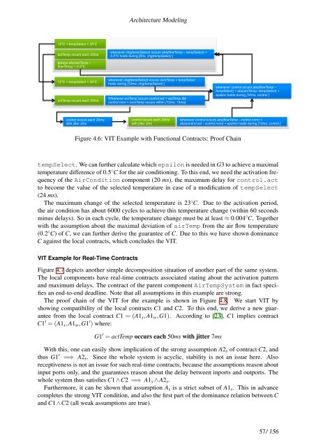
Figure 4.6: VIT Example with Functional Contracts: Proof Chain
tempSelect. We can further calculate which epsilon is needed in G3 to achieve a maximal
temperature difference of 0.5 ◦ C for the air conditioning. To this end, we need the activation frequency
of the AirCondition component (20 ms), the maximum delay for control.act
to become the value of the selected temperature in case of a modification of tempSelect
(24 ms).
The maximum change of the selected temperature is 23 ◦ C. Due to the activation period,
the air condition has about 6000 cycles to achieve this temperature change (within 60 seconds
minus delays). So in each cycle, the temperature change must be at least ≈ 0.004 ◦ C. Together
with the assumption about the maximal deviation of airTemp from the air flow temperature
(0.2 ◦ C) of C, we can further derive the guarantee of C. Due to this we have shown dominance
C against the local contracts, which concludes the VIT.
VIT Example for Real-Time Contracts
Figure 4.7 depicts another simple decomposition situation of another part of the same system.
The local components have real-time contracts associated stating about the activation pattern
and maximum delays. The contract of the parent component AirTempSystem in fact specifies
an end-to-end deadline. Note that all assumptions in this example are strong.
The proof chain of the VIT for the example is shown in Figure 4.8. We start VIT by
showing compatibility of the local contracts C1 and C2. To this end, we derive a new guarantee
from the local contract C1 = (A1s,A1w,G1). According to [23], C1 implies contract
C1 ′ = (A1s,A1w,G1 ′ ) where:
G1 ′ = actTemp occurs each 50ms with jitter 7ms
With this, one can easily show implication of the strong assumption A2s of contract C2, and
thus G1 ′ =⇒ A2s. Since the whole system is acyclic, stability is not an issue here. Also
receptiveness is not an issue for such real-time contracts, because the assumptions reason about
input ports only, and the guarantees reason about the delay between inports and outports. The
whole system thus satisfies C1 ∧C2 =⇒ A1s ∧ A2s.
Furthermore, it can be shown that assumption As is a strict subset of A1s. This in advance
completes the strong VIT condition, and also the first part of the dominance relation between C
and C1 ∧C2 (all weak assumptions are true).
57/ 156