- Page 1 and 2:
Proceedings e report 67
- Page 3 and 4:
Wood science for conservation of cu
- Page 5 and 6:
SUMMARY Introduction ..............
- Page 7 and 8:
WOOD SCIENCE FOR CONSERVATION OF CU
- Page 9 and 10:
INTRODUCTION These proceedings of a
- Page 11 and 12:
WOOD SCIENCE FOR CONSERVATION OF CU
- Page 13:
(A) MATERIAL PROPERTIES
- Page 16 and 17:
SORPTION OF MOISTURE AND DIMENSIONA
- Page 18 and 19:
SORPTION OF MOISTURE AND DIMENSIONA
- Page 20 and 21:
SORPTION OF MOISTURE AND DIMENSIONA
- Page 22 and 23:
VIBRATIONAL PROPERTIES OF TROPICAL
- Page 24 and 25:
VIBRATIONAL PROPERTIES OF TROPICAL
- Page 26 and 27:
VIBRATIONAL PROPERTIES OF TROPICAL
- Page 28 and 29:
CREEP PROPERTIES OF HEAT TREATED WO
- Page 30 and 31:
CREEP PROPERTIES OF HEAT TREATED WO
- Page 32 and 33:
CREEP PROPERTIES OF HEAT TREATED WO
- Page 34 and 35:
MEASUREMENT OF THE ELASTIC PROPERTI
- Page 36 and 37:
ELASTIC PROPERTIES OF MINUTE SAMPLE
- Page 38 and 39:
4. Results Young's modulus (10^4 Mp
- Page 40 and 41:
PREDICTION OF LINEAR DIMENSIONAL CH
- Page 42 and 43:
DIMENSIONAL CHANGE OF UNRESTRICTED
- Page 44 and 45:
DIMENSIONAL CHANGE OF UNRESTRICTED
- Page 46 and 47:
AGEING OF WOOD - DESCRIBED BY THE A
- Page 48 and 49:
AGEING OF WOOD - DESCRIBED BY THE A
- Page 50 and 51:
AGEING OF WOOD - DESCRIBED BY THE A
- Page 52 and 53:
90 30 0 3,0E-03 - 2,0E 2,0E-03 - 1,
- Page 54 and 55:
4. Application HYGRO-LOCK INTEGRATI
- Page 56 and 57:
RESEARCH ON THE AGING OF WOOD IN RI
- Page 58 and 59:
RESEARCH ON THE AGING OF WOOD IN RI
- Page 60 and 61:
Xylarium Database RESEARCH ON THE A
- Page 62 and 63:
AGING WOOD FROM CULTURAL PROPERTIES
- Page 64 and 65:
AGING WOOD FROM CULTURAL PROPERTIES
- Page 66 and 67:
STRENGTH AND MOE OF POPLAR WOOD (PO
- Page 68 and 69:
STRENGTH AND MOE OF POPLAR WOOD ACR
- Page 70 and 71:
STRENGTH AND MOE OF POPLAR WOOD ACR
- Page 72 and 73:
PHOTODEGRADATION AND THERMAL DEGRAD
- Page 74 and 75:
PHOTODEGRADATION AND THERMAL DEGRAD
- Page 76 and 77:
PHOTODEGRADATION AND THERMAL DEGRAD
- Page 79 and 80:
ROMANIAN WOODEN CHURCHES WALL PAINT
- Page 81 and 82:
WOOD SCIENCE FOR CONSERVATION OF CU
- Page 83 and 84:
WOOD SCIENCE FOR CONSERVATION OF CU
- Page 85 and 86:
DISINFECTION AND CONSOLIDATION BY I
- Page 87 and 88:
3. Results and discussion WOOD SCIE
- Page 89 and 90:
WOOD SCIENCE FOR CONSERVATION OF CU
- Page 91 and 92:
WOOD SCIENCE FOR CONSERVATION OF CU
- Page 93 and 94:
WOOD SCIENCE FOR CONSERVATION OF CU
- Page 95 and 96:
WOOD SCIENCE FOR CONSERVATION OF CU
- Page 97 and 98:
WOOD SCIENCE FOR CONSERVATION OF CU
- Page 99 and 100:
WOOD SCIENCE FOR CONSERVATION OF CU
- Page 101 and 102:
WOOD SCIENCE FOR CONSERVATION OF CU
- Page 103 and 104:
WOOD SCIENCE FOR CONSERVATION OF CU
- Page 105 and 106:
FUNGAL DECONTAMINATION BY COLD PLAS
- Page 107 and 108:
WOOD SCIENCE FOR CONSERVATION OF CU
- Page 109 and 110:
WOOD SCIENCE FOR CONSERVATION OF CU
- Page 111 and 112:
WOOD SCIENCE FOR CONSERVATION OF CU
- Page 113 and 114:
WOOD SCIENCE FOR CONSERVATION OF CU
- Page 115 and 116:
STUDIES ON INSECT DAMAGES OF WOODEN
- Page 117 and 118:
WOOD SCIENCE FOR CONSERVATION OF CU
- Page 119 and 120:
WOOD SCIENCE FOR CONSERVATION OF CU
- Page 121 and 122:
TERMITE INFESTATION RISK IN PORTUGU
- Page 123 and 124:
WOOD SCIENCE FOR CONSERVATION OF CU
- Page 125 and 126:
WOOD SCIENCE FOR CONSERVATION OF CU
- Page 127 and 128:
BIODETERIORATION OF CULTURAL HERITA
- Page 129 and 130: WOOD SCIENCE FOR CONSERVATION OF CU
- Page 131 and 132: 4. Causes of biodeterioration WOOD
- Page 133 and 134: DEGRADATION OF MELANIN AND BIOCIDES
- Page 135 and 136: WOOD SCIENCE FOR CONSERVATION OF CU
- Page 137 and 138: WOOD SCIENCE FOR CONSERVATION OF CU
- Page 139 and 140: MOULD ON ORGANS AND CULTURAL HERITA
- Page 141 and 142: WOOD SCIENCE FOR CONSERVATION OF CU
- Page 143 and 144: WOOD SCIENCE FOR CONSERVATION OF CU
- Page 145 and 146: WOOD SCIENCE FOR CONSERVATION OF CU
- Page 147 and 148: WOOD SCIENCE FOR CONSERVATION OF CU
- Page 149 and 150: WOOD SCIENCE FOR CONSERVATION OF CU
- Page 151 and 152: WOOD SCIENCE FOR CONSERVATION OF CU
- Page 153 and 154: WOOD SCIENCE FOR CONSERVATION OF CU
- Page 155 and 156: WOOD SCIENCE FOR CONSERVATION OF CU
- Page 157 and 158: RESEARCH STUDY ON THE EFFECTS OF TH
- Page 159 and 160: 4. Methodology WOOD SCIENCE FOR CON
- Page 161: WOOD SCIENCE FOR CONSERVATION OF CU
- Page 165 and 166: NON DESTRUCTIVE IMAGING FOR WOOD ID
- Page 167 and 168: METHODS OF NON-DESTRUCTIVE WOOD TES
- Page 169 and 170: WOOD SCIENCE FOR CONSERVATION OF CU
- Page 171 and 172: WOOD SCIENCE FOR CONSERVATION OF CU
- Page 173 and 174: MEASUREMENT AND SIMULATION OF DIMEN
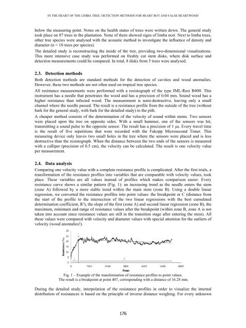
- Page 175 and 176: WOOD SCIENCE FOR CONSERVATION OF CU
- Page 177 and 178: WOOD SCIENCE FOR CONSERVATION OF CU
- Page 179: IN THE HEART OF THE LIMBA TREE (TER
- Page 183 and 184: WOOD SCIENCE FOR CONSERVATION OF CU
- Page 185 and 186: WOOD SCIENCE FOR CONSERVATION OF CU
- Page 187 and 188: WOOD SCIENCE FOR CONSERVATION OF CU
- Page 189 and 190: 3. Conclusions WOOD SCIENCE FOR CON
- Page 191 and 192: 2. Materials and methods WOOD SCIEN
- Page 193 and 194: WOOD SCIENCE FOR CONSERVATION OF CU
- Page 195 and 196: WOOD SCIENCE FOR CONSERVATION OF CU
- Page 197 and 198: 3. Chemometrics WOOD SCIENCE FOR CO
- Page 199 and 200: WOOD SCIENCE FOR CONSERVATION OF CU
- Page 201 and 202: 3. Results and discussion WOOD SCIE
- Page 203 and 204: NIR SPECTROSCOPIC MONITORING OF WAT
- Page 205 and 206: WOOD SCIENCE FOR CONSERVATION OF CU
- Page 207 and 208: NUMERICAL SIMULATION OF THE STRENGT
- Page 209 and 210: 3. Methods and models WOOD SCIENCE
- Page 211 and 212: WOOD SCIENCE FOR CONSERVATION OF CU
- Page 213 and 214: SIMPLE ELECTRONIC SPECKLE PATTERN I
- Page 215 and 216: WOOD SCIENCE FOR CONSERVATION OF CU
- Page 217 and 218: 5. Conclusions WOOD SCIENCE FOR CON
- Page 219 and 220: WOOD SCIENCE FOR CONSERVATION OF CU
- Page 221 and 222: Average r adiated presure field (dB
- Page 223 and 224: EXPERIMENTAL AND NUMERICAL MECHANIC
- Page 225 and 226: WOOD SCIENCE FOR CONSERVATION OF CU
- Page 227 and 228: WOOD SCIENCE FOR CONSERVATION OF CU
- Page 229 and 230: EFFECT OF THERMAL TREATMENT ON STRU
- Page 231 and 232:
WOOD SCIENCE FOR CONSERVATION OF CU
- Page 233 and 234:
WOOD SCIENCE FOR CONSERVATION OF CU
- Page 235 and 236:
The aims of this work are to: WOOD
- Page 237 and 238:
ultramarine [bad] titanium white [m
- Page 239 and 240:
4. Conclusions chrome yellow WOOD S
- Page 241 and 242:
WOOD SCIENCE FOR CONSERVATION OF CU
- Page 243 and 244:
WOOD SCIENCE FOR CONSERVATION OF CU
- Page 245 and 246:
WOOD SCIENCE FOR CONSERVATION OF CU
- Page 247 and 248:
WOOD SCIENCE FOR CONSERVATION OF CU
- Page 249 and 250:
Fig. 7 - A soaked lamella clamped i
- Page 251 and 252:
WOOD SCIENCE FOR CONSERVATION OF CU
- Page 253:
(D) CONSERVATION
- Page 256 and 257:
EUROPEAN TECHNICAL COMMITTEE 346 -
- Page 258 and 259:
EUROPEAN TECHNICAL COMMITTEE 346 -
- Page 260 and 261:
EUROPEAN TECHNICAL COMMITTEE 346 -
- Page 262 and 263:
EUROPEAN TECHNICAL COMMITTEE 346 -
- Page 264 and 265:
THE WRECK OF VROUW MARIA - CURRENT
- Page 266 and 267:
THE WRECK OF VROUW MARIA - CURRENT
- Page 268 and 269:
THE WRECK OF VROUW MARIA - CURRENT
- Page 270 and 271:
ROMANIAN ARCHITECTURAL WOODEN CULTU
- Page 272 and 273:
ROMANIAN ARCHITECTURAL WOODEN CULTU
- Page 274 and 275:
ROMANIAN ARCHITECTURAL WOODEN CULTU
- Page 276 and 277:
RESSURREIÇÃO DE CRISTO - PANEL FR
- Page 278 and 279:
ON 18 TH- AND 19 TH- CENTURY SACRIS
- Page 280 and 281:
ON 18TH- AND 19TH- CENTURY SACRISTY
- Page 282 and 283:
ON 18TH- AND 19TH- CENTURY SACRISTY
- Page 284 and 285:
ON 18TH- AND 19TH- CENTURY SACRISTY
- Page 286 and 287:
DEFIBRING OF HISTORICAL ROOF BEAM C
- Page 288 and 289:
DEFIBRING OF HISTORICAL ROOF BEAM C
- Page 290 and 291:
DEFIBRING OF HISTORICAL ROOF BEAM C
- Page 292 and 293:
EXAMINATION AND CONSERVATION OF TWO
- Page 294 and 295:
EXAMINATION AND CONSERVATION OF TWO
- Page 296 and 297:
THE CONSEQUENCES OF WOODEN STRUCTUR
- Page 298 and 299:
CONSEQUENCES OF WOODEN STRUCTURES C
- Page 301 and 302:
WHAT ONE NEEDS TO KNOW FOR THE ASSE
- Page 303 and 304:
WOOD SCIENCE FOR CONSERVATION OF CU
- Page 305 and 306:
WOOD SCIENCE FOR CONSERVATION OF CU
- Page 307 and 308:
WOOD SCIENCE FOR CONSERVATION OF CU
- Page 309 and 310:
WOOD SCIENCE FOR CONSERVATION OF CU
- Page 311 and 312:
load (KN) Samples 6 5 4 3 2 1 WOOD
- Page 313 and 314:
STRUCTURAL BEHAVIOUR OF TRADITIONAL
- Page 315 and 316:
WOOD SCIENCE FOR CONSERVATION OF CU
- Page 317 and 318:
WOOD SCIENCE FOR CONSERVATION OF CU
- Page 319 and 320:
WOOD SCIENCE FOR CONSERVATION OF CU
- Page 321 and 322:
WOOD SCIENCE FOR CONSERVATION OF CU
- Page 323 and 324:
WOOD SCIENCE FOR CONSERVATION OF CU
- Page 325:
WOOD SCIENCE FOR CONSERVATION OF CU
- Page 329 and 330:
INVESTIGATION ON THE UTILIZATION OF
- Page 331 and 332:
WOOD SCIENCE FOR CONSERVATION OF CU
- Page 333 and 334:
WOOD SCIENCE FOR CONSERVATION OF CU
- Page 335 and 336:
WOOD SCIENCE FOR CONSERVATION OF CU
- Page 337 and 338:
3. Results and discussions WOOD SCI
- Page 339 and 340:
WOOD SCIENCE FOR CONSERVATION OF CU
- Page 341:
Abadlia ......................... 3
- Page 345 and 346:
ANNEX 1: FACTS ABOUT COST ACTION IE
- Page 347 and 348:
WOOD SCIENCE FOR CONSERVATION OF CU
- Page 349 and 350:
WOOD SCIENCE FOR CONSERVATION OF CU
- Page 351 and 352:
Keynote presentations WOOD SCIENCE
- Page 353 and 354:
WOOD SCIENCE FOR CONSERVATION OF CU
- Page 355 and 356:
WOOD SCIENCE FOR CONSERVATION OF CU
- Page 357 and 358:
WOOD SCIENCE FOR CONSERVATION OF CU
- Page 359 and 360:
WOOD SCIENCE FOR CONSERVATION OF CU
- Page 362:
Finito di stampare presso Grafiche