Impact Of Host Plant Xylem Fluid On Xylella Fastidiosa Multiplication ...

The state variables, process functions and parameters are defined in Table 1. We emphasize that this model is in an early
development stage, and undoubtedly will evolve and improve as we develop it further. We used the delay-differential
equation (DDE) formalism developed by Murdoch et al. (1987) and Murdoch et al. (2003) for stage structured insects, and to
their formulation we will add time dependence (temperature forcing) of the developmental delays (although for simplicity we
will not elaborate on this here). The time dependence in the delays can be incorporated according to the mathematical recipes
developed by Nisbet and Gurney (1983), Gurney et al. (1983), Gurney and Nisbet (1998) and Nisbet (1998). Methods for
setting up the initial history for starting the models are outlined well in Gurney et al. (1983). We will solve our set of
equations using a new delay differential equation (DDE) solver, ddesd.m, (with time and system varying delays) developed
for The Mathworks (Matlab) by L. F. Shampine (Shampine & Thompson 2001, Shampine 2004). The solver is not yet a part
of Matlab itself, but a version is available on the Web at: http://faculty.smu.edu/lshampin/current.html .
Our model system.
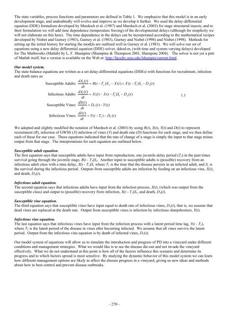
The state balance equations are written as a set delay-differential equations (DDEs) with functions for recruitment, infection
and death rates as:
dAS
() t
Susceptible Adults: = Rt ( −TJ) SJ − X( t) + X( t−T1) S1−DA( t)
dt
dAI
() t
Infectious Adults: = Xt ( ) −Xt ( −TS 1) 1−DA( t)
1.1
dt
dS()
t
Susceptible Vines: = DV
() t −Y()
t
dt
dI()
t
Infectious Vines: = Yt ( −T2
) −DV
( t)
dt
We adopted and slightly modified the notation of Murdoch et al. (2003) by using R(t), X(t), Y(t) and D(t) to represent
recruitment (R), infection of GWSS (X) infection of vines (Y) and death rate (D) functions for each stage, and we then define
each of these for our case. These equations indicated that the rate of change of a stage is simply the input to that stage minus
output from that stage. The interpretations for each equation are outlined below.
Susceptible adult equation.
The first equation says that susceptible adults have input from reproduction, one juvenile delay period (T J ) in the past times
survival going through the juvenile stage, R(t - T J )S J . Another input to susceptible adults is (possible) recovery from an
infectious adult class with a time delay, X(t - T 1 )S 1 where T 1 is the time that the disease persists in an infected adult, and S 1 is
the survival during the infectious period. Outputs from susceptible adults are infection by feeding on an infectious vine, X(t),
and death, D A (t).
Infectious adult equation.
The second equation says that infectious adults have input from the infection process, X(t), (which was output from the
susceptible class) and output to (possible) recovery from infection, X(t - T 1 )S 1 , and death, D A (t).
Susceptible vine equation.
The third equation says that susceptible vines have input equal to death rate of infectious vines, D V (t), that is, we assume that
dead vines are replaced at the death rate. Output from susceptible vines is infection by infectious sharpshooters, Y(t).
Infectious vine equation.
The last equation says that infectious vines have input from the infection process with a latent period time lag, Y(t - T 2 ),
where T 2 is the latent period of the disease in vines after becoming infected. We assume that all vines survive the latent
period. Output from the infectious vine equation is by death of infected vines, D V (t).
Our model system of equations will allow us to simulate the introduction and progress of PD into a vineyard under different
conditions and management strategies. What we would like is to see the disease die-out and not invade the vineyard
effectively. What we do not understand at this point is how all of the factors influence this scenario and determine its
progress and to which factors spread is most sensitive. By studying the dynamic behavior of this model system we can learn
how different management options are likely to affect the disease progress in a vineyard, giving us new ideas and methods
about how to best control and prevent disease outbreaks.
- 270 -