- Page 2 and 3:
UNIVERSITY OF HONG KOHG LlBEAEY
- Page 5 and 6:
International Conference on East As
- Page 7 and 8:
FOREWORD The International Conferen
- Page 10 and 11:
VHI LIST OF PARTICIPANTS IN THE PHO
- Page 12 and 13:
45 LIM, Hock National University of
- Page 15:
XIII INTERNATIONAL ORGANIZING COMMI
- Page 18 and 19:
XV! The mean heat sources over Asia
- Page 20 and 21:
XVIII , Jhe impact of urbanization
- Page 22 and 23:
XX The East Asia heavy rainfall num
- Page 24 and 25:
THE THERMAL STRUCTURE AND CONVECTIV
- Page 26 and 27:
THE COUPLING OF UPPER-LEVEL AND LOW
- Page 28 and 29:
Q \ ed atmospheric processes * 2. M
- Page 30 and 31:
2) DH Experiment The horizontal flo
- Page 32 and 33:
of the orography, establishing a na
- Page 34:
11 a o 12 21 36 4$ 60 fZ Pig.3. Nea
- Page 37 and 38:
14 OVERVIB/V CF MEI-YU RESEARCH IN
- Page 39 and 40:
16 Fig.l Climatological daily rainf
- Page 41 and 42:
18 showed a marked contrast between
- Page 43 and 44:
20 3. SWDPTiC ^mLYSIS WD DIA^DSTIC
- Page 45 and 46:
22 and Chang (27). It was also foun
- Page 47 and 48:
24 triggering mechanisms. In additi
- Page 49 and 50:
26 important mechanism for creating
- Page 51 and 52:
28 mature convections. Satellite pi
- Page 53 and 54:
30 States included 70 scientists an
- Page 55 and 56:
1-4 M-H C CO *+-« C CD 4-9 C o •
- Page 57 and 58:
34 19.Chen, G.T. J., "A study on sy
- Page 59 and 60:
36 complexes: 27-28 May 1981 case",
- Page 61 and 62:
38 On Temporal Variations of Low Le
- Page 63 and 64:
40 low-level flows of the Asian sum
- Page 65 and 66:
42 the northern part of the Pacific
- Page 67 and 68:
44 cycle is observed for the amplit
- Page 69 and 70:
46 SUMMER (6-85 : 12 2 M979 P:850 M
- Page 71 and 72:
Observed Structure and Propagation
- Page 73 and 74:
50 southeasterly current in the wes
- Page 75 and 76:
40°N 30°N 15°N Equator 90°E 105
- Page 77 and 78:
54 The pattern of arrows in Fig. 3
- Page 79 and 80:
56 Figure 5. Vertical cross-section
- Page 81 and 82:
58 TOE MEAN HEAT SOURCES OVER ASIAN
- Page 83 and 84:
60 over tost parts of India, Southe
- Page 85 and 86:
62 inctly different types. One is t
- Page 87 and 88:
64 60 70 too no 120 00
- Page 89 and 90:
Fig.2.The 7-month mean values of (a
- Page 91 and 92:
68 A NUMERICAL SIMULATION OF THE ME
- Page 93 and 94:
70 Synoptic circulation patterns fo
- Page 95 and 96:
72 (iii) The mid-latitude westerlie
- Page 97 and 98:
74 and the temperate latitude weste
- Page 99 and 100:
76 O 1 - (b) Total I Rainf a" 4 0
- Page 101 and 102:
78 LONGITUDE TIME WINOCROS5 SECTION
- Page 103 and 104:
A simulation of Lee-Cyclogenesis ov
- Page 105 and 106:
82 implemented to the global model
- Page 107 and 108:
84 In all three experiments, a deep
- Page 109:
86 References: Ballish, A.B., 1980:
- Page 116 and 117:
93 1.2-a I2.S 120. 127,5 US. 11.5 7
- Page 118 and 119:
95 2. Climatology of East Asian mon
- Page 120 and 121:
97 850 MB WIND (U*. V) S. 0 30N i~^
- Page 122 and 123:
99 120 ISO ISO 210 2VJ 770 ISO 180
- Page 124 and 125:
Figure 6 (a) Time-longitude section
- Page 126 and 127:
103 Monsoon cyclones /-~N I Subtrop
- Page 128 and 129:
105 INFLUENCE OF VARIATIONS OF THE
- Page 130 and 131:
surface during the rainy period of
- Page 132 and 133:
located at the position of the firs
- Page 134 and 135:
egion of western Australia. These t
- Page 138:
115 Fig.^57 Characteristics of vari
- Page 142 and 143:
119 Some Dynamic Aspects of the Equ
- Page 144 and 145:
121 equatorial zonal plane. In this
- Page 146 and 147:
123 where N is nondimensional Newto
- Page 148 and 149:
125 moisture concentration graduall
- Page 150 and 151:
127 boundary layer frictional conve
- Page 152 and 153:
129 000 - 20 30 WAVELENGTH (10 3 KM
- Page 154 and 155:
131 CHINESE POLAR ORBITING METEOROL
- Page 156 and 157:
some middle and small receiving sta
- Page 158:
135 local meteorology units through
- Page 163 and 164:
140 The Mesoscale Monitoring System
- Page 165 and 166:
142 The weather radar network is co
- Page 167 and 168:
144 where V and L are in centimeter
- Page 169 and 170:
146 PRF: 80-2000 Hz Minimum detecta
- Page 171 and 172:
148 [UHF Doppler RadaT] ^Pibalk ' Z
- Page 173 and 174:
150 STRUCTURAL FEATURES OF A SQUALL
- Page 175 and 176:
152 25 2200L 16 MAY 0000 L 17 MAY X
- Page 177 and 178:
154 0*73 KN 0,73 KM TAMEX IOF2 00*1
- Page 179 and 180:
156 4.2 East-west Cross Section The
- Page 181 and 182:
158 KM -20 EAST OF TOGA -10 0043 28
- Page 183 and 184:
160 Radar Observation of Precipitat
- Page 185 and 186:
162 Fig. 2. A triple doppler networ
- Page 187 and 188:
164 for this presentation Fig. 5a(0
- Page 189 and 190:
166 near the northern tip of Taiwan
- Page 191 and 192:
168 In order to understand the inte
- Page 193 and 194:
170 REMOTE SENSING OF ATMOSPHERIC C
- Page 195 and 196:
172 In the meantime, with the incre
- Page 197 and 198:
174 method (scanning frequency) and
- Page 199 and 200:
176 For sharp absorption lines, the
- Page 201 and 202:
178 [10]* Sun Jinhui, Qiu Jinhuan e
- Page 203 and 204:
180 COMPARISION OF RADAR ESTIMATES
- Page 205 and 206:
182 of 29 %). The Ra/Rg and the rel
- Page 207 and 208:
184 under 1) errors in estimating r
- Page 209 and 210:
186 Table 1. Summary of Ra/Rg for t
- Page 211 and 212:
188 FIGURE 3. CORRELATION COEFFICIE
- Page 213 and 214:
190 DOPPLER WEATHER RADAR OBSERVATI
- Page 215 and 216:
192 which are concerned about by th
- Page 217 and 218:
194 fly on schedule, take off and l
- Page 219 and 220:
196 and minus value. Fig. 4 is the
- Page 221 and 222:
198 REFERENCES 1. Donald Turnbull e
- Page 223 and 224:
200 evaporation, condensation, wind
- Page 225 and 226:
202 control valve which permits amp
- Page 227 and 228:
204 Table 1 Rainfall Records of a T
- Page 229 and 230:
206 various rainfall intensity shou
- Page 231 and 232:
208 c 400-- £ o "5 350 H — A —
- Page 233 and 234:
210 IMPACT OF HOURLY S-VISSR SATELL
- Page 235 and 236:
212 Fig. 1. Daily 1.200 UTC • 500
- Page 237 and 238:
I Fig. 2. GMS-3 IR picture taken at
- Page 239 and 240:
216 110E 20 115E 30. 20" X J 4o*N'\
- Page 241 and 242:
218 Fig. 7. Provisional best track
- Page 243 and 244:
220 PREDICTABILITY OF LOW FREQUENCY
- Page 245 and 246:
222 expressions that invoke the Mon
- Page 247 and 248:
224 b) A low frequency mode experim
- Page 249 and 250:
226 A CLOUD WAVE THEORY AND ITS APP
- Page 251 and 252:
228 heating indicating a substantia
- Page 253 and 254:
230 If N Fig. I, A schematic diagra
- Page 255 and 256:
232 2. A Quasi-Diabatic Geostrophic
- Page 257 and 258:
234 X can be q, £ c, v, or T. The
- Page 259 and 260:
236 On the basis of the preceding d
- Page 261 and 262:
238 west of the maximum cloud cover
- Page 263 and 264:
240 NORMAL MODES OF CLIMATOLOGICAL
- Page 265 and 266:
242 (1983) pointed out that simulat
- Page 267 and 268:
244 reach the top of model atmosphe
- Page 269 and 270:
246 is not clear in the tropics. Th
- Page 271 and 272:
248 Wang, J.-T., J.-W. Kim and W.L.
- Page 273 and 274:
250 (a) 30°N-30°S (January) (b) 3
- Page 275 and 276:
252 An Important element of the ear
- Page 277 and 278:
254 IOCS I02S 3SN Fig. 1 A general
- Page 279 and 280:
256 staion of LID (farmland in the
- Page 281 and 282:
258 start from October 1990 and end
- Page 283 and 284:
260 The measurements of surface rad
- Page 285 and 286:
262 Secular trends in urban tempera
- Page 287 and 288:
264 LONGTERM TEMPERATURE TRENDS AT
- Page 289 and 290:
266 Using these data sources It has
- Page 291 and 292:
268 (3) a nearly static phase where
- Page 293 and 294:
270 greater rate of increasing mini
- Page 295 and 296:
272 consistent with accepted theory
- Page 297 and 298:
274 RECENT APPLICATIONS OF THE PENN
- Page 299 and 300:
276 upward motion (Fig. Ib) of air
- Page 301 and 302:
278 Stauffer and Warner (1987) used
- Page 303 and 304:
280 observed precipitation rates fo
- Page 305 and 306:
282 coupled model system show that
- Page 307 and 308:
284 Baroclinic Instability of Modif
- Page 309 and 310:
286 Eq (2.4) corresponds to the con
- Page 311 and 312:
288 conventional Eady waves, except
- Page 313 and 314:
290 perturbations in Mode I remains
- Page 315 and 316:
292 5: Summary And Remarks Two diff
- Page 317 and 318:
294 INFLUENCES OF OROGRAPHY ON FLOW
- Page 319 and 320:
296 (13) The next step is to determ
- Page 321 and 322:
298 where „ = 1 - R a = - R 2>x c
- Page 323 and 324:
300 — -~ 1, thus the above relati
- Page 325 and 326:
302 The vertical velocity at the to
- Page 327 and 328:
304 THE MIGEOPHYSICS OF A MEI-YU CA
- Page 329 and 330:
306 O.Qg-m" 3 , which is probably d
- Page 331 and 332:
308 snowflakes aggregation generate
- Page 333 and 334:
310 (a) TRP.CK - 2 (1652 0 - 1711 0
- Page 335 and 336:
312 1987 6/16 17QSSO U 0.9 C 2 = 1.
- Page 337 and 338:
314 2. Heavy Rainfall Upstream of a
- Page 339 and 340:
316 accumulated rainfall amount on
- Page 341 and 342:
318 Figures 11 and 12 demonstrate t
- Page 343 and 344:
320 DEGREE K IT ( M/S ) QC (G/KG) -
- Page 345 and 346:
322 270 290 310 330 350 370 POTJEMP
- Page 347 and 348:
324 A primitive equation model was
- Page 349 and 350:
326 had already been affected by so
- Page 351 and 352:
328 I .011 I 1...J/1 l\l l-L-l L I
- Page 353 and 354:
330 «'.. Fig. 11 Same as Fig. 9 ex
- Page 355 and 356:
332 Mathiar, M. B., 1983: A quasi-L
- Page 357 and 358:
334 Long (1985), the maximum occure
- Page 359 and 360:
336 February 1979. It clearly indic
- Page 361 and 362:
338 Jiang H. M. and Jeng H. N., "Nu
- Page 363 and 364:
TEMP.GRAD.(C/100KM3 1979/2/04/OOZ 1
- Page 365 and 366:
TKANS.C1R. 9 1979/2/04/OE2 •; J97
- Page 367 and 368:
344 however, the sharp decrease in
- Page 369 and 370:
346 00 " XD 3 b D 3 aD b dD = [ N.
- Page 371 and 372:
348 heights. The median diameter an
- Page 373 and 374:
350 going on within the melting lay
- Page 375 and 376:
352 TRFICK - I (HIS 0 - H31 0J PR0B
- Page 377 and 378:
354 MONTHLY AND SEASONAL FORECASTS
- Page 379 and 380:
356 In another experiment, the heat
- Page 381 and 382:
358 4. CONCLUSION The forecasting e
- Page 383 and 384:
360 TABLE 1. COMPARISONS OF THE COR
- Page 385 and 386:
362 Fig. 3. Map of the correlation
- Page 387 and 388:
364 THE TELECONNECTION OF EQUATORIA
- Page 389 and 390:
366 3-*-j-] dag grid % ^Showing eve
- Page 391 and 392:
368 oBE (6) fl(uP) , fl(vP) ... 0(w
- Page 393 and 394:
370 the major tidal components over
- Page 395 and 396:
372 one meter. Most of the water le
- Page 397 and 398:
374 and Technology Advisory Group,
- Page 399 and 400:
376 INTRODUCTION In 1%6, Bjerknes,
- Page 401 and 402:
378 THE INTERANNUAL VARIABILITIES O
- Page 403 and 404:
380 current between 127° E—128°
- Page 405 and 406:
382 El Nino and Southern Oscillatio
- Page 407 and 408:
384 Fig.5. The ADCP measurements (s
- Page 409 and 410:
386 I. Introduction Climate is one
- Page 411 and 412:
388 specifically at the modeling an
- Page 413 and 414:
390 Even during the warm phase of t
- Page 415 and 416:
392 (iv) To investigate the morphol
- Page 417 and 418:
394 Change program under IGBP is a
- Page 419 and 420:
396 TABLE 1: PROCESSES TO BE STUDIE
- Page 421 and 422:
398 w / / / / / / / / /-"V / / Z Fi
- Page 423 and 424:
400 CHINA-JAPAN JOINT RESEARCH PROG
- Page 425 and 426:
402 eastward. In addition to mainta
- Page 427 and 428:
404 Processes of Hicroscale Air-Sea
- Page 429 and 430:
406 phase velocity; both ratios, th
- Page 431 and 432:
T i l l ! o I • GO 00 J Wind Velo
- Page 433 and 434:
410 Concluding Remarks In order to
- Page 435 and 436:
412 THE VARIATIONS OF THE SST IN TH
- Page 437 and 438:
414 maps, there is an extensive are
- Page 439 and 440:
416 Flg.1. Time series of the annua
- Page 441 and 442:
418 90 N 90 S|. . . 20E 20E Fig.3c.
- Page 443 and 444:
420 ON LABORATORY SIMULATION OF SEA
- Page 445 and 446:
422 EXPERIMENT: Only simple and eas
- Page 447 and 448:
424 With the ability to simulate co
- Page 449 and 450:
426 (5) Meroney, R.N., Cermak, J.E.
- Page 451 and 452:
428 Fig. 3 Composite Photograph of
- Page 453 and 454:
430 A detailed description of the m
- Page 455 and 456:
432 However, the schemes failed to
- Page 457 and 458:
434 REFERENCES Anderson, E. and A.
- Page 459 and 460:
436 Figure 2 Vertical structure of
- Page 461 and 462:
438 36 HOUR FORECAST MEAN SEA LEVEL
- Page 463 and 464:
440 al.,1984). In this paper, a gen
- Page 465 and 466:
442 where subscript x denotes u, v,
- Page 467 and 468:
444 AM AM PO- N3 A/i + N3' and NH--
- Page 469 and 470:
446 there is only a minor differenc
- Page 471 and 472:
448 Guo X.R.,Yan Z.H.,Zhang Y.L. an
- Page 473 and 474:
450 THE EAST ASIA HEAVY RAINFALL NU
- Page 475 and 476:
452 (described in section 2) carrie
- Page 477 and 478:
454 Fig. . 2. Validation of Tempera
- Page 479 and 480:
456 simulate the partly cloudy cond
- Page 481 and 482: 458 3.3 Nesting Run with 2 km Grids
- Page 483 and 484: 460 REFERENCES Bhumralker, C. M., 1
- Page 485 and 486: 462 The Impact of the Termination o
- Page 487 and 488: 464 and 45.8 km respectively, which
- Page 489 and 490: 466 relative to (P+O/2, they actual
- Page 491 and 492: 468 Chang, S. W., 1982: The ore-gra
- Page 493 and 494: 470 Table 3. 24-hour forecast error
- Page 495 and 496: 472 Initial Position Errors 1983-19
- Page 497 and 498: 474 A SPECTRAL MODEL FOR MEDIUM RAN
- Page 499 and 500: 476 where I p u = FC-
- Page 501 and 502: 478 given. This is treated separate
- Page 503 and 504: 480 predicted location is too far t
- Page 505 and 506: 482 Fig.2 Distribution of 24h preci
- Page 507 and 508: 484 LONG-RANGE FORECASTING OF TAIWA
- Page 509 and 510: 486 monsoon in east Asia and for co
- Page 511 and 512: 488 unfortunately are not integral
- Page 513 and 514: Figure 1. SPECTRAL ANALYSIS FOR MAY
- Page 515 and 516: 492 TaUj.g_ji Multiple rnfjross i o
- Page 517 and 518: 494 THE NONLINEAR INTERACTION OF IN
- Page 519 and 520: 496 Burgers(l948) had put forward a
- Page 521 and 522: 498 From Eqs,(8), the necessary con
- Page 523 and 524: 500 In order to show quantitatively
- Page 525 and 526: 502 Multiple Equilibria Of a Therma
- Page 527 and 528: 504 For the two-level quasi-geostro
- Page 529 and 530: 506 The coefficients Z, T, H, and T
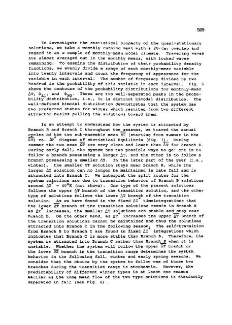
- Page 531: 508 just the stable Branch 7 for st
- Page 535 and 536: 512 STATIONARY SOLUTIONS WITH TOPOG
- Page 537 and 538: 514 ANNTTAL CYCLE OF 2TTT Fig. 7 An
- Page 539 and 540: 516 CISK modes have narrow axes of
- Page 541 and 542: 518 about one to three weeks. Predi
- Page 543 and 544: 520 first one. In his work, the lon
- Page 545 and 546: 522 The works mentioned are qualita
- Page 547 and 548: 524 [12] Wang, S.-W., Adv. in Atmos
- Page 549 and 550: 526 processes that give rise to a d
- Page 551 and 552: 528 3 Local energetics analysis The
- Page 553 and 554: 530 dominant waves of a local mode
- Page 555 and 556: 532 slightly longer than the length
- Page 557 and 558: 534 tends to induce a westerly jet
- Page 559 and 560: 536 TYPHOON FORMATION AND DEVELOPME
- Page 561 and 562: 538 influence of the mean wind prof
- Page 563 and 564: 540 3. Steady-State Solutions The p
- Page 565 and 566: 542 of maximum wind (Fig 7 c). This
- Page 567 and 568: 544 (A) b- l.O.(B) b- 0.8.(C) b- 0.
- Page 569 and 570: 546 b= 1.0,C= 0.03,0 = 120., T = 50
- Page 571 and 572: 548 tropical cyclones. Then, Shapir
- Page 573 and 574: 550 fine equation (2) will be used
- Page 575 and 576: 552 4) Cumulus vertical flux of hea
- Page 577 and 578: 554 Fig. 4 Same as Fig, 1, but for
- Page 579 and 580: 556 n=800 bPa and r **1. Now it is
- Page 581 and 582: 558 RRFKRRNCF Challa, M., and R. T,
- Page 583 and 584:
560 The limited-area forecast syste
- Page 585 and 586:
562 Our study is to obtain and anal
- Page 587 and 588:
564 coarse grid (Fig. 5). The struc
- Page 589 and 590:
566 ACCUMULATED PRECIPITATION Fig.
- Page 592 and 593:
569 AUTHOR INDEX ANTHES, Richard A.
- Page 594 and 595:
571 LIOU, Chi-Sann LIU, Cho-Teng LI