Каталог Weidmuller: Electronics - Analogue Signal Conditioning

Derating curve (current-carrying capacity curve)
Electrical data
Technical appendix/Glossary
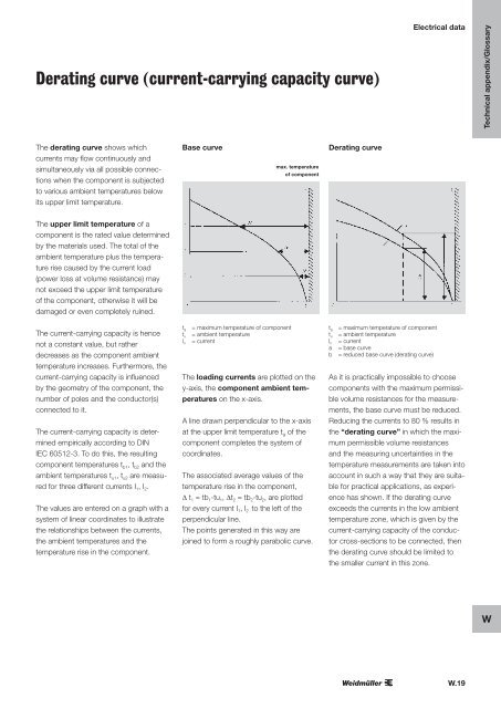
The derating curve shows which
currents may flow continuously and
simultaneously via all possible connections
when the component is subjected
to various ambient temperatures below
its upper limit temperature.
Base curve
max. temperature
of component
Derating curve
The upper limit temperature of a
component is the rated value determined
by the materials used. The total of the
ambient temperature plus the temperature
rise caused by the current load
(power loss at volume resistance) may
not exceed the upper limit temperature
of the component, otherwise it will be
damaged or even completely ruined.
The current-carrying capacity is hence
not a constant value, but rather
decreases as the component ambient
temperature increases. Furthermore, the
current-carrying capacity is influenced
by the geometry of the component, the
number of poles and the conductor(s)
connected to it.
The current-carrying capacity is determined
empirically according to DIN
IEC 60512-3. To do this, the resulting
component temperatures t b1 , t b2 and the
ambient temperatures t u1 , t u2 are measured
for three different currents I 1 , I 2 .
The values are entered on a graph with a
system of linear coordinates to illustrate
the relationships between the currents,
the ambient temperatures and the
temperature rise in the component.
t g = maximum temperature of component
t u = ambient temperature
I n = current
The loading currents are plotted on the
y-axis, the component ambient temperatures
on the x-axis.
A line drawn perpendicular to the x-axis
at the upper limit temperature t g of the
component completes the system of
coordinates.
The associated average values of the
temperature rise in the component,
Δ t 1 = tb 1 -tu 1 , Δt 2 = tb 2 -tu 2 , are plotted
for every current I 1 , I 2 to the left of the
perpendicular line.
The points generated in this way are
joined to form a roughly parabolic curve.
t g = maximum temperature of component
t u = ambient temperature
I n = current
a = base curve
b = reduced base curve (derating curve)
As it is practically impossible to choose
components with the maximum permissible
volume resistances for the measurements,
the base curve must be reduced.
Reducing the currents to 80 % results in
the “derating curve” in which the maximum
permissible volume resistances
and the measuring uncertainties in the
temperature measurements are taken into
account in such a way that they are suitable
for practical applications, as experience
has shown. If the derating curve
exceeds the currents in the low ambient
temperature zone, which is given by the
current-carrying capacity of the conductor
cross-sections to be connected, then
the derating curve should be limited to
the smaller current in this zone.
W
W.19