- Page 1:
AgroindustrialProjectAnalysis James
- Page 5 and 6:
AgroindustrialProject AnalysisJames
- Page 7 and 8:
ContentsForeword by Ajit MozoomdarP
- Page 10 and 11:
ForewordAGROINDUSTRY-that is, indus
- Page 12 and 13:
XPREFACEThe following colleagues ga
- Page 15 and 16:
IAn OverviewTHE PURPOSE OF THIS BOO
- Page 17 and 18:
AN OVERVIEW 5ing factory must conte
- Page 19 and 20:
AN OVERVIEW 7trialization occurs ca
- Page 21 and 22:
AN OVERVIEW 9Table 1-2. Contributio
- Page 23 and 24: AN OVERVIEW 11cent; this far exceed
- Page 25 and 26: AN OVERVIEW 13By broadening its agr
- Page 27 and 28: AN OVERVIEW 15agroindustries from i
- Page 29 and 30: AN OVERVIEW 17focus than indicated
- Page 31 and 32: AN OVERVIEW 19be interested in cost
- Page 33 and 34: AN OVERVIEW 21that warrant further
- Page 35 and 36: AN OVERVIEW 23prises of different s
- Page 37 and 38: AN OVERVIEW 25an interactive proces
- Page 39 and 40: 2The Marketing FactorTHE VIABILITY
- Page 41 and 42: THE MARKETING FACTOR 29testing cons
- Page 43 and 44: THE MARKETING FACTOR 31product to t
- Page 45 and 46: Figure 4. Illustrative Segmentation
- Page 47 and 48: THE MARKETING FACTOR 35ucts are pur
- Page 49 and 50: THE MARKETING FACTOR 37decisionmaki
- Page 51 and 52: THE MARKETING FACTOR 39gional, nati
- Page 53 and 54: Figure 5. Product Life Cycle (PLC)M
- Page 55 and 56: THE MARKETING FACTOR 43Institutiona
- Page 57 and 58: THE MARKETING FACTOR 45How do insti
- Page 59 and 60: THE MARKETING FACTOR 47ssl's may ne
- Page 61 and 62: THE MARKETING FACTOR 49the governme
- Page 63 and 64: THE MARKETING FACTOR 51consciousnes
- Page 65 and 66: THE MARKETING FACTOR 53FUNCTIONS. M
- Page 67 and 68: THE MARKETING FACTOR 55the processo
- Page 69 and 70: THE MARKETING FACTOR 57Responses by
- Page 71 and 72: THE MARKETING FACTOR 59* Likely com
- Page 73: THE MARKETING FACTOR 61Table 2-3. T
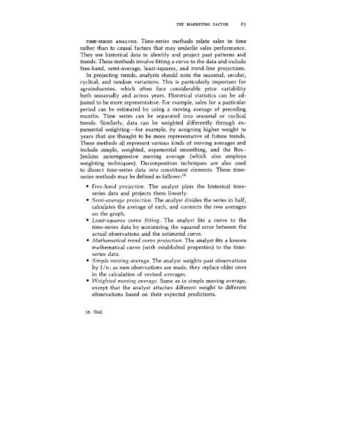
- Page 77 and 78: THE MARKETING FACTOR 65ence of appr
- Page 79 and 80: THE MARKETING FACTOR 67Are the data
- Page 81 and 82: THE MARKETING FACTOR 69ect's market
- Page 83 and 84: THE PROCUREMENT FACTOR 71* Cost. Th
- Page 85 and 86: THE PROCUREMENT FACTOR 73the declin
- Page 87 and 88: TIIE PROCUREMENT FACTOR 75termine t
- Page 89 and 90: THE PROCUREMENT FACTOR 77C- cost pe
- Page 91 and 92: THE PROCUREMENT FACTOR 79Figure 7.
- Page 93 and 94: TBE PROCUREMENT FACTOR8itomato crop
- Page 95 and 96: THE PROCUREMENT FACTOR 83Storage an
- Page 97 and 98: THE PROCUREMENT FACTOR 85Is there c
- Page 99 and 100: THE PROCUREMENT FACTOR 87desired re
- Page 101 and 102: THE PROCUREMENT FACTOR 89of the qua
- Page 103 and 104: THE PROCUREMENT FACTOR 91Even with
- Page 105 and 106: THE PROCUREMENT FACTOR 93The firm s
- Page 107 and 108: THE PROCUREMENT FACTOR 95A crop's a
- Page 109 and 110: THE PROCUREMENT FACTOR 97Table 3-4.
- Page 111 and 112: THE PROCUREMENT FACTOR 99the transp
- Page 113 and 114: THE PROCUREMENT FACTOR 101credit or
- Page 115 and 116: THE PROCUREMENT FACTOR 103firm's pr
- Page 117 and 118: THE PROCUREMENT FACTOR 105Are multi
- Page 119 and 120: THE PROCUREMENT FACTOR 107Seeds and
- Page 121 and 122: THE PROCUREMENT FACTOR 109tion. Inc
- Page 123 and 124: THE PROCUREMENT FACTOR 111size; emp
- Page 125 and 126:
THE PROCUREMENT FACTOR 113Salient p
- Page 127 and 128:
THE PROCUREMENT FACTOR 115storage a
- Page 129 and 130:
4The Processing FactorTHis STUDY HA
- Page 131 and 132:
THE PROCESSING FACTOR 119In milling
- Page 133 and 134:
THE PROCESSING FACTOR 121tion that
- Page 135 and 136:
n.a., Not applicable.Source: C. Pet
- Page 137 and 138:
THE PROCESSING FACTOR 125labor perm
- Page 139 and 140:
THE PROCESSING FACTOR 127tions have
- Page 141 and 142:
THE PROCESSING FACTOR 129season. Fi
- Page 143 and 144:
THE PROCESSING FACTOR 131sensitive
- Page 145 and 146:
THE PROCESSING FACTOR 133Table 4-4.
- Page 147 and 148:
THE PROCESSING FACTOR 135soluble nu
- Page 149 and 150:
THE PROCESSING FACTOR 137Food Produ
- Page 151 and 152:
THE PROCESSING FACTOR 139* Fragile
- Page 153 and 154:
THE PROCESSING FACTOR 141* Availabi
- Page 155 and 156:
THE PROCESSING FACTOR 143the cost o
- Page 157 and 158:
THE PROCESSING FACTOR 145cessor in
- Page 159 and 160:
THE PROCESSING FACTOR 14715 percent
- Page 161 and 162:
THE PROCESSING FACTOR 149and A. The
- Page 163 and 164:
THE PROCESSING FACTOR 151example, i
- Page 165 and 166:
THE PROCESSING FACTOR 153primary in
- Page 167 and 168:
THE PROCESSING FACTOR 155For more c
- Page 169 and 170:
THE PROCESSING FACTOR 157farmer's a
- Page 171 and 172:
THE PROCESSING FACTOR 159failed to
- Page 173 and 174:
THE PROCESSING FACTOR 16rbecause of
- Page 175 and 176:
COSTS OF ALTERNATIVE TECHNOLOGY 163
- Page 177 and 178:
COSTS OF ALTERNATIVE TECHNOLOGY 165
- Page 179 and 180:
can process almost any eration); $0
- Page 181 and 182:
Pneumatic Batch or continuous $120,
- Page 183 and 184:
of previously driedproducts; best f
- Page 185 and 186:
Fluidized Continuous operation $372
- Page 187 and 188:
Plate Batch operation for $372,000
- Page 189 and 190:
system cookers (probably simi- to t
- Page 191 and 192:
CHECKLIST OF CRITICAL QUESTIONS 179
- Page 193 and 194:
CHECKLIST OF CRITICAL QUESTIONS 18I
- Page 195 and 196:
CHECKLIST OF CRITICAL QUESTIONS 183
- Page 197 and 198:
CHECKLIST OF CRITICAL QUESTIONS 185
- Page 199 and 200:
CHECKLIST OF CRITICAL QUESTIONS 187
- Page 201 and 202:
CHECKLIST OF CRITICAL QUESTIONS 189
- Page 203 and 204:
CHECKLIST OF CRITICAL QUESTIONS 191
- Page 205 and 206:
CHECKLIST OF CRITICAL QUESTIONS 193
- Page 207 and 208:
CHECKLIST OF CRITICAL QUESTIONS 195
- Page 209 and 210:
CHECKLIST OF CRITICAL QUESTIONS 197
- Page 211 and 212:
BibliographyTHE FOLLOWING WORKS AUG
- Page 213 and 214:
BiBLIOGRAPHY 201Scott, M., J. D. Ma
- Page 215 and 216:
BIBLIOGRAPHY 203Forecasting methods
- Page 217 and 218:
BIBLIOGRAPHY 205UNIDO. UNIDO Guides
- Page 219 and 220:
BIBLIOGRAPHY 207tional Affairs, no.
- Page 221 and 222:
IndexAdvertising, 42, 128; promotio
- Page 223 and 224:
INDEX 211development planning and,
- Page 225 and 226:
INDEX 213Social costs and benefits:
- Page 228:
The World BankEconomic Development


![Problem 1: Loop Unrolling [18 points] In this problem, we will use the ...](https://img.yumpu.com/36629594/1/184x260/problem-1-loop-unrolling-18-points-in-this-problem-we-will-use-the-.jpg?quality=85)