- Page 2:
THE SCIENCE ANDAPPLICATIONS OFACOUS
- Page 8 and 9:
xPrefaceReferencesBacon, Sir Franci
- Page 10 and 11:
xiiContents16. Ultrasonics 44317. C
- Page 12:
2 1. A Capsule History of Acoustics
- Page 15 and 16:
1. A Capsule History of Acoustics 5
- Page 17 and 18:
1. A Capsule History of Acoustics 7
- Page 19:
1. A Capsule History of Acoustics 9
- Page 22 and 23:
12 1. A Capsule History of Acoustic
- Page 24 and 25:
14 2. Fundamentals of AcousticsFigu
- Page 26 and 27:
16 2. Fundamentals of Acoustics2.2
- Page 28 and 29:
18 2. Fundamentals of Acousticsof t
- Page 30 and 31:
20 2. Fundamentals of AcousticsQ z+
- Page 32 and 33:
22 2. Fundamentals of Acousticsin t
- Page 34 and 35:
24 2. Fundamentals of AcousticsWe c
- Page 36 and 37:
26 2. Fundamentals of Acoustics(2)
- Page 38 and 39:
28 2. Fundamentals of AcousticsEqua
- Page 40 and 41:
30 2. Fundamentals of Acoustics11.
- Page 42 and 43:
32 3. Sound Wave Propagation and Ch
- Page 44 and 45:
34 3. Sound Wave Propagation and Ch
- Page 46 and 47:
36 3. Sound Wave Propagation and Ch
- Page 48 and 49:
38 3. Sound Wave Propagation and Ch
- Page 50 and 51:
40 3. Sound Wave Propagation and Ch
- Page 52 and 53:
42 3. Sound Wave Propagation and Ch
- Page 54 and 55:
44 3. Sound Wave Propagation and Ch
- Page 56 and 57:
46 3. Sound Wave Propagation and Ch
- Page 58 and 59:
48 3. Sound Wave Propagation and Ch
- Page 60 and 61:
50 3. Sound Wave Propagation and Ch
- Page 62:
52 3. Sound Wave Propagation and Ch
- Page 65 and 66:
3.14 Performance Indices for Enviro
- Page 67 and 68:
3.14 Performance Indices for Enviro
- Page 69 and 70:
or in terms of complex exponential
- Page 71 and 72:
3.17 Sound Intensity 61Here the sur
- Page 73 and 74:
3.18 The Monopole Source 63The thre
- Page 75 and 76:
3.21 Energy Density 653.20 The Hemi
- Page 77 and 78:
References 67medium. The time avera
- Page 79 and 80:
Problems for Chapter 3 69(a) the wa
- Page 81 and 82:
4Vibrating Strings4.1 IntroductionI
- Page 83 and 84:
4.4 General Solution of the Wave Eq
- Page 85 and 86:
4.6 Simple Harmonic Solutions of th
- Page 87 and 88:
4.7 Standing Waves 77Figure 4.3. Di
- Page 89 and 90:
4.8 The Effect of Initial Condition
- Page 91 and 92:
4.10 Forced Vibrations in an Infini
- Page 93 and 94:
4.11 Strings of Finite Lengths: For
- Page 95 and 96:
References 854.12 Real Strings: Fre
- Page 97 and 98:
Problems for Chapter 4 878. A devic
- Page 99 and 100:
90 5. Vibrating BarsFigure 5.1. A b
- Page 101 and 102:
92 5. Vibrating BarsSettingc 2 = E/
- Page 103 and 104:
94 5. Vibrating BarsThe allowable f
- Page 105 and 106:
96 5. Vibrating Barsthe acceleratio
- Page 107 and 108:
98 5. Vibrating BarsFigure 5.5. Loc
- Page 109 and 110:
100 5. Vibrating Barsmore difficult
- Page 111 and 112:
102 5. Vibrating BarsFigure 5.7. An
- Page 113 and 114:
104 5. Vibrating Barsthe light beam
- Page 115 and 116:
106 5. Vibrating BarsFigure 5.8. Tr
- Page 117 and 118:
108 5. Vibrating BarsFigure 5.10. T
- Page 119 and 120:
110 5. Vibrating Barsof 0.005 m dia
- Page 121 and 122:
112 6. Membrane and PlatesFigure 6.
- Page 123 and 124:
114 6. Membrane and PlatesBecause t
- Page 125 and 126:
116 6. Membrane and PlatesThe left-
- Page 127 and 128:
118 6. Membrane and PlatesTable 6.1
- Page 129 and 130:
120 6. Membrane and PlatesIn real a
- Page 131 and 132:
122 6. Membrane and PlatesTable 6.2
- Page 133 and 134:
124 6. Membrane and PlatesAt low fr
- Page 135 and 136:
126 6. Membrane and PlatesThe elast
- Page 137 and 138:
128 6. Membrane and PlatesFor the f
- Page 139 and 140:
130 6. Membrane and Plates(b) Deter
- Page 141 and 142:
132 7. Pipes, Waveguides, and Reson
- Page 143 and 144:
134 7. Pipes, Waveguides, and Reson
- Page 145 and 146:
136 7. Pipes, Waveguides, and Reson
- Page 147 and 148:
138 7. Pipes, Waveguides, and Reson
- Page 149 and 150:
140 7. Pipes, Waveguides, and Reson
- Page 151 and 152:
142 7. Pipes, Waveguides, and Reson
- Page 153 and 154:
144 7. Pipes, Waveguides, and Reson
- Page 155 and 156:
146 7. Pipes, Waveguides, and Reson
- Page 157 and 158:
148 7. Pipes, Waveguides, and Reson
- Page 159 and 160:
150 7. Pipes, Waveguides, and Reson
- Page 161 and 162:
152 8. Acoustic Analogs, Ducts, and
- Page 163 and 164:
154 8. Acoustic Analogs, Ducts, and
- Page 165 and 166:
156 8. Acoustic Analogs, Ducts, and
- Page 167 and 168:
158 8. Acoustic Analogs, Ducts, and
- Page 169 and 170:
160 8. Acoustic Analogs, Ducts, and
- Page 171 and 172:
162 8. Acoustic Analogs, Ducts, and
- Page 173 and 174:
164 8. Acoustic Analogs, Ducts, and
- Page 175 and 176:
166 8. Acoustic Analogs, Ducts, and
- Page 177 and 178:
168 8. Acoustic Analogs, Ducts, and
- Page 179 and 180:
170 8. Acoustic Analogs, Ducts, and
- Page 181 and 182:
9Sound-Measuring Instrumentation9.1
- Page 183 and 184:
9.3 Microphones 175Figure 9.1. A cu
- Page 185 and 186:
SolutionEquation (9.3) is applied t
- Page 187 and 188:
9.5 Selection and Positioning of Mi
- Page 189 and 190:
9.6 Vector Sound Intensity Probes 1
- Page 191 and 192:
9.8 Proper Procedures for Using the
- Page 193 and 194:
9.8 Proper Procedures for Using the
- Page 195 and 196:
Example Problem 39.10 Dosimeters 18
- Page 197 and 198:
9.11 Noise Measurement in Selected
- Page 199 and 200:
9.11 Noise Measurement in Selected
- Page 201 and 202:
9.12 Real Time Analysis 193analyzer
- Page 203 and 204:
9.13 Fast Fourier Transform Analysi
- Page 205 and 206:
9.14 Data Windows and Selection of
- Page 207 and 208:
9.16 Measurement Error 199whereβ =
- Page 209 and 210:
9.18 Measurement of Sound in a Free
- Page 211 and 212:
9.20 Sound Power Measurement in a D
- Page 213 and 214:
9.20 Sound Power Measurement in a D
- Page 215 and 216:
9.23 The Addition Method for Measur
- Page 217 and 218:
References 209acoustical output and
- Page 219 and 220:
Problems for Chapter 9 2112. Determ
- Page 221 and 222:
214 10. Physiology of Hearing and P
- Page 223 and 224:
216 10. Physiology of Hearing and P
- Page 225 and 226:
218 10. Physiology of Hearing and P
- Page 227 and 228:
220 10. Physiology of Hearing and P
- Page 229 and 230:
222 10. Physiology of Hearing and P
- Page 231 and 232:
224 10. Physiology of Hearing and P
- Page 233 and 234:
226 10. Physiology of Hearing and P
- Page 235 and 236:
228 10. Physiology of Hearing and P
- Page 237 and 238:
230 10. Physiology of Hearing and P
- Page 239 and 240:
232 10. Physiology of Hearing and P
- Page 241 and 242:
234 10. Physiology of Hearing and P
- Page 243 and 244:
236 10. Physiology of Hearing and P
- Page 245 and 246:
238 10. Physiology of Hearing and P
- Page 247 and 248:
240 10. Physiology of Hearing and P
- Page 249 and 250: 11Acoustics of Enclosed Spaces:Arch
- Page 251 and 252: 11.2 Sound Fields 245Figure 11.1. P
- Page 253 and 254: 11.4 Sound Intensity Growth in a Li
- Page 255 and 256: 11.5 Sound Absorption Coefficients
- Page 257 and 258: 11.6 Growth of Sound with Absorbent
- Page 259 and 260: 11.7 Decay of Sound 253Following Sa
- Page 261 and 262: 11.8 Decay of Sound in Dead Rooms 2
- Page 263 and 264: 11.9 Reverberation as Affected by S
- Page 265 and 266: 11.13 Sound Levels due to Direct an
- Page 267 and 268: 11.15 Concert Halls and Opera House
- Page 269 and 270: Figure 11.9. A view of the Boston S
- Page 271 and 272: 11.15 Concert Halls and Opera House
- Page 273 and 274: 11.15 Concert Halls and Opera House
- Page 275 and 276: 11.15 Concert Halls and Opera House
- Page 277 and 278: 11.16 Band Shells and Outdoor Audit
- Page 279 and 280: 11.16 Band Shells and Outdoor Audit
- Page 281 and 282: 11.17 Subjective Preferences in Sou
- Page 283 and 284: References 277preferred subsequent
- Page 285 and 286: Problems for Chapter 11 279Siebein,
- Page 287 and 288: 12Walls, Enclosures, and Barriers12
- Page 289 and 290: 12.3 Mass Control Case 283Figure 12
- Page 291 and 292: 12.5 Effect of Frequencies on Sound
- Page 293 and 294: 12.6 Coincidence Effect and Critica
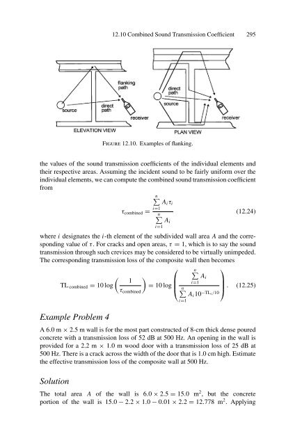
- Page 295 and 296: 12.7 The Double-Panel Partition 289
- Page 297 and 298: an ideal gas) varies in the followi
- Page 299: 12.8 Measuring Transmission Loss 29
- Page 303 and 304: 12.11 Noise Insulation Ratings 297F
- Page 305 and 306: 12.11 Noise Insulation Ratings 299s
- Page 307 and 308: 12.12 Noise Reduction of a Wall 301
- Page 309 and 310: 12.12 Noise Reduction of a Wall 303
- Page 311 and 312: 12.14 Enclosures 305to the extent t
- Page 313 and 314: 12.14 Enclosures 307and similarly f
- Page 315 and 316: 12.15 Small Enclosures 309walls. Ac
- Page 317 and 318: 12.16 Acoustic Barriers 311Figure 1
- Page 319 and 320: 12.16 Acoustic Barriers 313In the c
- Page 321 and 322: Equation (12.67) becomes(11D = λ+
- Page 323 and 324: Problems for Chapter 12 3173. A 0.7
- Page 325 and 326: 13Criteria and Regulations forNoise
- Page 327 and 328: 13.3 The Occupational Safety and He
- Page 329 and 330: 13.4 Perception of Noise 323inspect
- Page 331 and 332: 13.6 Indoor Noise Criteria 325accou
- Page 333 and 334: 13.6 Indoor Noise Criteria 327Room
- Page 335 and 336: 13.7 Equivalent Sound Level, Day-Ni
- Page 337 and 338: 13.7 Equivalent Sound Level, Day-Ni
- Page 339 and 340: Composite Noise Rating13.9 Rating o
- Page 341 and 342: 13.10 Evaluation of Traffic Noise 3
- Page 343 and 344: 13.10 Evaluation of Traffic Noise 3
- Page 345 and 346: Highway Construction Noise13.10 Eva
- Page 347 and 348: 13.10 Evaluation of Traffic Noise 3
- Page 349 and 350: 13.10 Evaluation of Traffic Noise 3
- Page 351 and 352:
13.11 Evaluation of Community Noise
- Page 353 and 354:
13.12 Guidelines and Regulations in
- Page 355 and 356:
13.12 Guidelines and Regulations in
- Page 357 and 358:
13.12 Guidelines and Regulations in
- Page 359 and 360:
References 353Computer Program, HIC
- Page 361 and 362:
Problems for Chapter 13 355Problems
- Page 363 and 364:
14Machinery Noise Control14.1 Intro
- Page 365 and 366:
14.4 Fan or Blower Noise 359Table 1
- Page 367 and 368:
14.4 Fan or Blower Noise 361Figure
- Page 369 and 370:
14.4 Fan or Blower Noise 363Table 1
- Page 371 and 372:
14.4 Fan or Blower Noise 365Table 1
- Page 373 and 374:
14.6 Pumps and Plumbing Systems 367
- Page 375 and 376:
14.6 Pumps and Plumbing Systems 369
- Page 377 and 378:
14.8 Gears 371fromwheref BRC = N r
- Page 379 and 380:
14.8 Gears 373Figure 14.7. Gear noi
- Page 381 and 382:
14.8 Gears 375Figure 14.8. Gear tra
- Page 383 and 384:
14.8 Gears 377The subscripts 1 and
- Page 385 and 386:
14.10 Ball and Roller Bearings 379l
- Page 387 and 388:
14.10 Ball and Roller Bearings 381c
- Page 389 and 390:
14.11 Other Mechanical Drive Elemen
- Page 391 and 392:
Belt Drivesf CL = n 1N 1 2400 × 12
- Page 393 and 394:
14.12 Gas-Jet Noise 387said to be c
- Page 395 and 396:
14.12 Gas-Jet Noise 389power discha
- Page 397 and 398:
Solution14.12 Gas-Jet Noise 391Usin
- Page 399 and 400:
14.13 Gas Jet Noise Control 393Solu
- Page 401 and 402:
14.13 Gas Jet Noise Control 395Figu
- Page 403 and 404:
14.13 Gas Jet Noise Control 397Figu
- Page 405 and 406:
14.14 Mufflers and Silencers 399Fig
- Page 407 and 408:
(1 + m)A I 1=A 314.14 Mufflers and
- Page 409 and 410:
14.14 Mufflers and Silencers 403Let
- Page 411 and 412:
References 405Figure 14.21 illustra
- Page 413 and 414:
Problems for Chapter 14 407the nois
- Page 415 and 416:
15Underwater Acoustics15.1 Sound Pr
- Page 417 and 418:
15.3 Speed of Sound in Seawater 411
- Page 419 and 420:
15.4 Velocity Profiles in the Sea 4
- Page 421 and 422:
15.4 Velocity Profiles in the Sea 4
- Page 423 and 424:
15.5 Underwater Transmission Loss 4
- Page 425 and 426:
15.6 Parametric Variation of Absorp
- Page 427 and 428:
15.8 Underwater Refraction 421Figur
- Page 429 and 430:
15.9 Mixed Layer 423When G is const
- Page 431 and 432:
15.11 Sonar Transducers and Their P
- Page 433 and 434:
Example Problem 115.12 The Sonar Eq
- Page 435 and 436:
Active and Passive Equations15.12 T
- Page 437 and 438:
15.13 Noise, Echo, and Reverberatio
- Page 439 and 440:
15.13 Noise, Echo, and Reverberatio
- Page 441 and 442:
15.14 Transient Form of Sonar Equat
- Page 443 and 444:
Example Problem 315.16 Shortcomings
- Page 445 and 446:
15.17 Theoretical Target Strength o
- Page 447 and 448:
Problems for Chapter 15 441Wilson,
- Page 449 and 450:
444 16. Ultrasonicscatching small i
- Page 451 and 452:
446 16. UltrasonicsPlanck constant
- Page 453 and 454:
448 16. UltrasonicsEquation (16.5)
- Page 455 and 456:
450 16. UltrasonicsFigure 16.1. Sou
- Page 457 and 458:
452 16. Ultrasonicsthe positive hal
- Page 459 and 460:
454 16. Ultrasonicson each and ever
- Page 461 and 462:
456 16. Ultrasonicscomplete as a li
- Page 463 and 464:
458 16. Ultrasonicsinitial of their
- Page 465 and 466:
460 16. Ultrasonicsoptic axis, deno
- Page 467 and 468:
462 16. Ultrasonicstransducer, it h
- Page 469 and 470:
464 16. UltrasonicsTable 16.1. Valu
- Page 471 and 472:
466 16. Ultrasonicsthe mechanical r
- Page 473 and 474:
468 16. UltrasonicsThe Physics of M
- Page 475 and 476:
470 16. UltrasonicsFigure 16.7. The
- Page 477 and 478:
472 16. Ultrasonicscurvilinear arra
- Page 479 and 480:
474 16. Ultrasonics(a)amplitudeinpu
- Page 481 and 482:
476 16. Ultrasonicsslow to allow th
- Page 483 and 484:
478 16. Ultrasonics5. In the cases
- Page 485 and 486:
480 17. Commercial and Medical Ultr
- Page 487 and 488:
482 17. Commercial and Medical Ultr
- Page 489 and 490:
484 17. Commercial and Medical Ultr
- Page 491 and 492:
486 17. Commercial and Medical Ultr
- Page 493 and 494:
488 17. Commercial and Medical Ultr
- Page 495 and 496:
490 17. Commercial and Medical Ultr
- Page 497 and 498:
492 17. Commercial and Medical Ultr
- Page 499 and 500:
494 17. Commercial and Medical Ultr
- Page 501 and 502:
496 17. Commercial and Medical Ultr
- Page 503 and 504:
498 17. Commercial and Medical Ultr
- Page 505 and 506:
500 17. Commercial and Medical Ultr
- Page 507 and 508:
502 17. Commercial and Medical Ultr
- Page 509 and 510:
504 17. Commercial and Medical Ultr
- Page 511 and 512:
506 17. Commercial and Medical Ultr
- Page 513 and 514:
508 17. Commercial and Medical Ultr
- Page 515 and 516:
510 18. Music and Musical Instrumen
- Page 517 and 518:
512 18. Music and Musical Instrumen
- Page 519 and 520:
Figure 18.7. The frequencies of the
- Page 521 and 522:
516 18. Music and Musical Instrumen
- Page 523 and 524:
518 18. Music and Musical Instrumen
- Page 525 and 526:
520 18. Music and Musical Instrumen
- Page 527 and 528:
522 18. Music and Musical Instrumen
- Page 529 and 530:
524 18. Music and Musical Instrumen
- Page 531 and 532:
526 18. Music and Musical Instrumen
- Page 533 and 534:
528 18. Music and Musical Instrumen
- Page 535 and 536:
530 18. Music and Musical Instrumen
- Page 537 and 538:
532 18. Music and Musical Instrumen
- Page 539 and 540:
Figure 18.20. The violin octet deve
- Page 541 and 542:
536 18. Music and Musical Instrumen
- Page 543 and 544:
538 18. Music and Musical Instrumen
- Page 545 and 546:
540 18. Music and Musical Instrumen
- Page 547 and 548:
542 18. Music and Musical Instrumen
- Page 549 and 550:
544 18. Music and Musical Instrumen
- Page 551 and 552:
546 18. Music and Musical Instrumen
- Page 553 and 554:
548 18. Music and Musical Instrumen
- Page 555 and 556:
550 18. Music and Musical Instrumen
- Page 557 and 558:
552 18. Music and Musical Instrumen
- Page 559 and 560:
554 18. Music and Musical Instrumen
- Page 561 and 562:
556 18. Music and Musical Instrumen
- Page 563 and 564:
558 18. Music and Musical Instrumen
- Page 565 and 566:
560 18. Music and Musical Instrumen
- Page 567 and 568:
562 18. Music and Musical Instrumen
- Page 569 and 570:
564 18. Music and Musical Instrumen
- Page 571 and 572:
566 18. Music and Musical Instrumen
- Page 573 and 574:
568 18. Music and Musical Instrumen
- Page 575 and 576:
570 19. Sound ReproductionAlbert, a
- Page 577 and 578:
572 19. Sound ReproductionD. Magnet
- Page 579 and 580:
574 19. Sound Reproductionon, machi
- Page 581 and 582:
576 19. Sound ReproductionIt is fai
- Page 583 and 584:
578 19. Sound ReproductionINNER SUS
- Page 585 and 586:
580 19. Sound Reproductiontuned ape
- Page 587 and 588:
582 19. Sound Reproductionuse of MP
- Page 589 and 590:
584 19. Sound ReproductionDickason,
- Page 591 and 592:
586 20. Vibration and Vibration Con
- Page 593 and 594:
588 20. Vibration and Vibration Con
- Page 595 and 596:
590 20. Vibration and Vibration Con
- Page 597 and 598:
592 20. Vibration and Vibration Con
- Page 599 and 600:
594 20. Vibration and Vibration Con
- Page 601 and 602:
596 20. Vibration and Vibration Con
- Page 603 and 604:
598 20. Vibration and Vibration Con
- Page 605 and 606:
600 20. Vibration and Vibration Con
- Page 607 and 608:
602 20. Vibration and Vibration Con
- Page 609 and 610:
604 20. Vibration and Vibration Con
- Page 611 and 612:
606 20. Vibration and Vibration Con
- Page 613 and 614:
608 20. Vibration and Vibration Con
- Page 615 and 616:
610 20. Vibration and Vibration Con
- Page 617 and 618:
612 20. Vibration and Vibration Con
- Page 619 and 620:
614 20. Vibration and Vibration Con
- Page 621 and 622:
616 20. Vibration and Vibration Con
- Page 623 and 624:
618 21. Nonlinear Acousticsby∇ 2
- Page 625 and 626:
620 21. Nonlinear Acousticsmay be i
- Page 627 and 628:
622 21. Nonlinear Acousticswhereδ
- Page 629 and 630:
624 21. Nonlinear AcousticsThe shoc
- Page 631 and 632:
626 21. Nonlinear AcousticsBut the
- Page 633 and 634:
Appendix APhysical Properties of Ma
- Page 635 and 636:
Appendix A. Physical Properties of
- Page 637 and 638:
Appendix BBessel FunctionsB.1 The B
- Page 639 and 640:
B.8 Tables of Bessel Functions, Zer
- Page 641 and 642:
Appendix CUsing Laplace Transforms
- Page 643 and 644:
C.3 Solving Differential Equations
- Page 645 and 646:
C.4 Equations with Multiple-Order R
- Page 647 and 648:
SolutionC.5 Equations with Complex
- Page 649 and 650:
C.5 Equations with Complex Roots 64
- Page 651 and 652:
SolutionC.5 Equations with Complex
- Page 653 and 654:
650 IndexAuditoriums, design of, 26
- Page 655 and 656:
652 IndexElectrostatic speakers, 58
- Page 657 and 658:
654 IndexKey notation, 518Kinetic e
- Page 659 and 660:
656 IndexPascal (unit), 48Percent i
- Page 661 and 662:
658 IndexSound intensity growth in
- Page 663:
660 IndexWater-hammer arresters, 37