- Page 1:
XIII Advanced Research Workshop on
- Page 4 and 5:
� [539.12.01 + 539.12 ... 14
- Page 6 and 7:
Analytic perturbation theory and pr
- Page 8 and 9:
Measurements of GEp/GMp to high Q 2
- Page 11 and 12:
WELCOME ADDRESS Alexei Sissakian Di
- Page 13 and 14:
he joined the group of prof. Przemy
- Page 15 and 16:
proton. Dividing these 90 ◦ cm p-
- Page 17 and 18:
p-p scattering angle fixed at exact
- Page 19 and 20:
tuning for each ring. The Workshop
- Page 21 and 22:
was only about 10 5 per second, but
- Page 23:
[10] E.F. Parker et al., Phys. Rev.
- Page 27 and 28:
MICROSCOPIC STERN-GERLACH EFFECT AN
- Page 29 and 30:
DeGrand-Miettinen model predicted P
- Page 31 and 32:
TOWARDS STUDY OF LIGHT SCALAR MESON
- Page 33 and 34:
104xdBR(φ--> π η 0 -1 γ )/dm, G
- Page 35 and 36:
RECURSIVE FRAGMENTATION MODEL WITH
- Page 37 and 38:
Figure 2: String decaying into pseu
- Page 39 and 40:
pT -distributions in the quark frag
- Page 41 and 42:
4 Inclusion of spin-1 mesons For a
- Page 43 and 44:
CONSTITUENT QUARK REST ENERGY AND W
- Page 45 and 46:
〈r 2 ch 〉≈1fm2 . Now with Eqs
- Page 47 and 48:
TOWARDS A MODEL INDEPENDENT DETERMI
- Page 49 and 50:
Common for the difference cross sec
- Page 51 and 52:
TRANSVERSITY GPDs FROM γN → πρ
- Page 53 and 54:
The scattering amplitude of the pro
- Page 55 and 56:
INFRARED PROPERTIES OF THE SPIN STR
- Page 57 and 58:
5 Acknowledgement B.I. Ermolaev is
- Page 59 and 60:
We shall call this model the “sec
- Page 61 and 62:
y f ν V = f l V = f u V = f d gz V
- Page 63 and 64:
2. We remind, that the celebrated G
- Page 65 and 66:
of the resonance A, θV � 39 o .
- Page 67 and 68:
• Right-handed EW currents. The c
- Page 69 and 70:
pesum- (p Entries 0 + pe)-(p-pe) Me
- Page 71 and 72:
CROSS SECTIONS AND SPIN ASYMMETRIES
- Page 73 and 74:
R(ρ) 5 4 3 2 1 0 2 3 4 5 6 7 8 9 1
- Page 75 and 76:
TWO-PHOTON EXCHANGE IN ELASTIC ELEC
- Page 77 and 78:
and depend on three parameters : fN
- Page 79 and 80:
O(αs) SPIN EFFECTS IN e + e −
- Page 81 and 82:
3 Polarization results for mq → 0
- Page 83 and 84:
Since one has (↑↓) pc Born =(
- Page 85 and 86:
Figure 1: A typical lowest order Fe
- Page 87 and 88:
sin φ S (π + ) A UT 1.0 0.8 0.6 0
- Page 89 and 90:
form the agreement with these data
- Page 91 and 92:
in settling this dynamical issue. G
- Page 93 and 94:
SPIN CORRELATIONS OF THE ELECTRON A
- Page 95 and 96: the two-photon system equaling 1).
- Page 97 and 98: ANOTHER NEW TRACE FORMULA FOR THE C
- Page 99 and 100: Compare the gain of time and effort
- Page 101 and 102: where the triplet and octet axial c
- Page 103 and 104: [2] Y. Prok et al. [CLAS Collaborat
- Page 105 and 106: Melosh rotations which boost the re
- Page 107 and 108: ky �GeV� 0.4 0.2 0.0 �0.2 �
- Page 109 and 110: [2] B. Pasquini, and S. Boffi, Phys
- Page 111 and 112: The appearance of both |+〉 and |
- Page 113 and 114: 2.2 Intrinsic Transverse Motion Qua
- Page 115 and 116: are still complex: for a given corr
- Page 117 and 118: This last is required to complete t
- Page 119 and 120: [16] P.G. Ratcliffe and O.V. Teryae
- Page 121 and 122: Figure 1: a)[left] μpG p E /Gp M (
- Page 123 and 124: 4 Conclusion We introduced a simple
- Page 125 and 126: √ δΔq8 x for Δq8 and γΔGx fo
- Page 127 and 128: understanding of polarized light qu
- Page 129 and 130: They are inverse powers of Q 2 kine
- Page 131 and 132: accounts approximately for the TM a
- Page 133 and 134: POTENTIAL FOR A NEW MUON g-2 EXPERI
- Page 135 and 136: When the momentum increases (p >p0)
- Page 137 and 138: EVOLUTION EQUATIONS FOR TRUNCATED M
- Page 139 and 140: 4 Perspectives Evolution equations
- Page 141 and 142: NEW DEVELOPMENTS IN THE QUANTUM STA
- Page 143 and 144: statistical approach compared to th
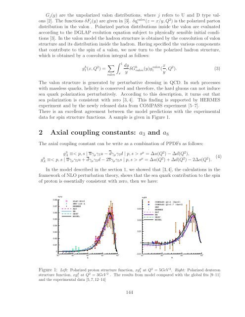
- Page 145: POLARIZED HADRON STRUCTURE IN THE V
- Page 149 and 150: AXIAL ANOMALIES, NUCLEON SPIN STRUC
- Page 151 and 152: 3. Vector current of strange quarks
- Page 153 and 154: ORBITAL MOMENTUM EFFECTS DUE TO A L
- Page 155 and 156: The elastic scattering S-matrix in
- Page 157 and 158: IDENTIFICATION OF EXTRA NEUTRAL GAU
- Page 159 and 160: for final l + l − events (l = μ,
- Page 161 and 162: QUARK INTRINSIC MOTION AND THE LINK
- Page 163 and 164: where wP = − m 2M 2 −p1 cos ω
- Page 165 and 166: where g q 2x − ξ 1(x, pT )= πM2
- Page 167: EXPERIMENTAL RESULTS
- Page 170 and 171: 01 00 11 01 01 01 00 11 01 01 01 00
- Page 172 and 173: where C1, C2 and A1 - signals from
- Page 174 and 175: Figure 1: Layout of experiment targ
- Page 176 and 177: According to requirements of the de
- Page 178 and 179: Electron energy is measured at ATLA
- Page 180 and 181: Fig. 2 shows the results of the lon
- Page 182 and 183: e γ* e’ x+ ξ x− ξ A A’ e e
- Page 184 and 185: cos 0φ C A φ cos C A cos 2φ C A
- Page 186 and 187: 5 Summary HERMES has measured signi
- Page 188 and 189: (1.205 ± 0.0012) GeV/c, 10 10 p/s,
- Page 190 and 191: was done in the interval ”−t”
- Page 192 and 193: If we admit a non-zero quark transv
- Page 194 and 195: which is trivial in collinear LO ap
- Page 196 and 197:
In figure 3 the expected errors on
- Page 198 and 199:
[12] A. V. Efremov and O. V. Teryae
- Page 200 and 201:
Figure 1: The COMPASS spectrometer.
- Page 202 and 203:
Comparing this formula to the inclu
- Page 204 and 205:
Figure 5: Comparison of COMPASS inc
- Page 206 and 207:
[9] B. Adeva et al. (SMC Coll.), Ph
- Page 208 and 209:
q T sin( φ-φ ) M AUT 0.14 0.12 0.
- Page 210 and 211:
proton beam is planned. References
- Page 212 and 213:
Run Year √ s (GeV) Polarization R
- Page 214 and 215:
ackground fraction, and asymmetry i
- Page 216 and 217:
At √ s = 200 GeV, ALL(pp → π
- Page 218 and 219:
[6] D. de Florian, W. Vogelsang, an
- Page 220 and 221:
higher energies, where the cross se
- Page 222 and 223:
Figure 3: The experimental results
- Page 224 and 225:
kinematic range to low values of Bj
- Page 226 and 227:
3 Semi-Inclusive DIS Collins and Si
- Page 228 and 229:
Unpolarized target asymmetries. The
- Page 230 and 231:
4 Summary Since the end of data-tak
- Page 232 and 233:
polarization as well as a construct
- Page 234 and 235:
Finally the COMPASS reconstruction
- Page 236 and 237:
tained in the NLO QCD approximation
- Page 238 and 239:
with only modern NN potential are r
- Page 240 and 241:
(a) (b) Figure 3: (a) T20 data take
- Page 242 and 243:
of electroproduction from polarized
- Page 244 and 245:
As is seen in Fig. 1 values of the
- Page 246 and 247:
SEMI-INCLUSIVE DIS AND TRANSVERSE M
- Page 248 and 249:
The yellow band in Fig. 1 is the re
- Page 250 and 251:
At leading twist, a third asymmetry
- Page 252 and 253:
THE COMPLETION OF SINGLE-SPIN ASYMM
- Page 254 and 255:
A N , % 30 20 10 0 0 0.2 0.4 0.6 0.
- Page 256 and 257:
Unexpectedly large single spin asym
- Page 258 and 259:
THE GENERALIZED PARTON DISTRIBUTION
- Page 260 and 261:
, E) H ~ (H, I Im C 5 4 3 2 1 Q = 1
- Page 262 and 263:
Reducing to a common denominator (
- Page 264 and 265:
LAMBDA PHYSICS AT HERMES S. Belosto
- Page 266 and 267:
analysis was carried out reconstruc
- Page 268 and 269:
SPIN PHYSICS AT NICA A. Nagaytsev J
- Page 270 and 271:
original software packages (MC simu
- Page 272 and 273:
MEASUREMENTS OF TRANSVERSE SPIN EFF
- Page 274 and 275:
to “near-side” and “away-side
- Page 276 and 277:
THE FIRST STAGE OF POLARIZATION PRO
- Page 278 and 279:
In paper [12] the study was made of
- Page 280 and 281:
emphasis to increase the statistics
- Page 282 and 283:
Table 2: The parameters of the main
- Page 284 and 285:
POLARIZATION MEASUREMENTS IN PHOTOP
- Page 286 and 287:
With a polarized electron beam inci
- Page 288 and 289:
Figure 3: Preliminary helicity asym
- Page 290 and 291:
INVESTIGATION OF DP-ELASTIC SCATTER
- Page 292 and 293:
framework with the use of deuteron
- Page 294 and 295:
SPIN PHYSICS WITH CLAS Y. Prok 12,
- Page 296 and 297:
1.3 Flavor Decomposition of the Hel
- Page 298 and 299:
Γ p 1 0.15 0.125 0.1 0.075 0.05 0.
- Page 300 and 301:
The upcoming energy upgrade of Jeff
- Page 302 and 303:
y the nearly 1000 combined citation
- Page 304 and 305:
� R = −Pt/Pl τ(1 + ε)/2ε; he
- Page 306 and 307:
4 Results of GEp-III Experiment In
- Page 308 and 309:
6 Theoretical Developments The earl
- Page 310 and 311:
lz = 0 (along the direction of the
- Page 312 and 313:
models have recently been challenge
- Page 314 and 315:
[32] Chung P. L. and F. Coester, Ph
- Page 316 and 317:
48 ± 3% for two beams. The proton
- Page 318 and 319:
is constant with cos θ∗ , as exp
- Page 320 and 321:
In summary, we made measurements on
- Page 322 and 323:
angle between the direction of the
- Page 324 and 325:
The sensitivity of the data to the
- Page 326 and 327:
COMPASS could be converted into a f
- Page 328 and 329:
3.1.2 Beam charge and spin asymmetr
- Page 330 and 331:
contributions enter only beyond lea
- Page 332 and 333:
References [1] D. Mueller et al, Fo
- Page 334 and 335:
l’ l p q p h H (z) 1 h (x) 1 l l
- Page 336 and 337:
3. Data selection. The data selecti
- Page 338 and 339:
φ sin3 a 0.06 0.04 0.02 0 -0.02 -0
- Page 340 and 341:
TRANSVERSE SPIN AND MOMENTUM EFFECT
- Page 342 and 343:
model. Both the cos φh and the cos
- Page 344 and 345:
D cos φ A 0 -0.1 -0.2 -0.3 + h -2
- Page 346 and 347:
4.3 The Sivers asymmetry According
- Page 348 and 349:
[3] A. Airapetian et al. [HERMES co
- Page 350 and 351:
2. Delta-Sigma Experimental Set-up.
- Page 352 and 353:
6. Estimate of the count rate in tr
- Page 354 and 355:
2 Analysis Formalism Spin-dependent
- Page 356 and 357:
The MC production comprises three s
- Page 358 and 359:
6 High pT hadron pair analysis for
- Page 360 and 361:
[2] V. Y. Alexakhin et al. [COMPASS
- Page 362 and 363:
2 Towards polarized Antiprotons For
- Page 364 and 365:
4 Spin-Filtering Experiments at COS
- Page 366 and 367:
to test the theoretical models of t
- Page 368 and 369:
C1 C2 π CH1,2 CH3,4 CH5,6 111 000
- Page 370 and 371:
not even resemble the data behavior
- Page 372 and 373:
to the slope of the Rosenbluth plot
- Page 374 and 375:
The differential cross section of t
- Page 376 and 377:
with zero for all mass ranges, with
- Page 378 and 379:
more precise and dedicated measurem
- Page 380 and 381:
oth types of experiment results are
- Page 382 and 383:
is recorded, a good particle identi
- Page 384 and 385:
error of the extracted asymmetries
- Page 386 and 387:
2.6 Summary and Outlook The first d
- Page 388 and 389:
386
- Page 391 and 392:
PROTON BEAM POLARIZATION MEASUREMEN
- Page 393:
N A 0.06 0.05 0.04 0.03 0.02 0.01 0
- Page 396 and 397:
Intensity profile (arb. units) 1 0.
- Page 398 and 399:
[4] H. Okada et al., Proc. of the 1
- Page 400 and 401:
The amplitudes of the signals and t
- Page 402 and 403:
The following results has been obta
- Page 404 and 405:
interaction vanishes and a single Z
- Page 406 and 407:
an amorphous NH3 for low and high,
- Page 408 and 409:
and depends on a choice of � ℓ1
- Page 410 and 411:
3 The conditions for transparent sp
- Page 412 and 413:
where angles α and β are defined
- Page 414 and 415:
forward angles, where vector Ay and
- Page 416 and 417:
espectively. The open symbols repre
- Page 418 and 419:
RF dipole (transverse B): εBdl = 1
- Page 420 and 421:
i PV / PV i PV / PV 1 0.5 0 -0.5 -1
- Page 422 and 423:
The energies of the states Ψ1 −
- Page 424 and 425:
field P ≈ +1. If we add the trans
- Page 426 and 427:
econstruction provide more accurate
- Page 428 and 429:
y detector saturation from pC colli
- Page 430 and 431:
2 �p+ 8 He analyzing power measur
- Page 432 and 433:
3.3 Effect of valence neutrons on s
- Page 434 and 435:
i.e. n0(θ +2π) =n0(θ) . There ar
- Page 436 and 437:
w and ˙ɛ. For example, we use par
- Page 438 and 439:
436
- Page 441 and 442:
REGULARIZATION OF SOURCE OF THE KER
- Page 443 and 444:
The corresponding phase transition
- Page 445 and 446:
ABOUT SPIN PARTICLE SOLUTION IN BOR
- Page 447 and 448:
where the functions fi(s, η) must
- Page 449 and 450:
SPINDYNAMICS I.B. Pestov JINR, 1419
- Page 451 and 452:
State of hadron matter is defined t
- Page 453 and 454:
REMARK ON SPIN PRECESSION FORMULAE
- Page 455 and 456:
It is easy to see that for a (massi
- Page 457 and 458:
DYNAMICS OF SPIN IN NONSTATIC SPACE
- Page 459 and 460:
Schwinger gauge. Probably for the f
- Page 461 and 462:
DSPIN-09 WORKSHOP SUMMARY Jacques S
- Page 463 and 464:
to some preliminary results reporte
- Page 465 and 466:
A new measurement of the polarizati
- Page 467 and 468:
new NLO QCD parametrization of the
- Page 469:
Name (Institution, Town, Country) E