XI Seminario de Investigación - Facultad de IngenierÃa - Universidad ...
XI Seminario de Investigación - Facultad de IngenierÃa - Universidad ...
XI Seminario de Investigación - Facultad de IngenierÃa - Universidad ...

Create successful ePaper yourself
Turn your PDF publications into a flip-book with our unique Google optimized e-Paper software.
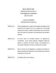
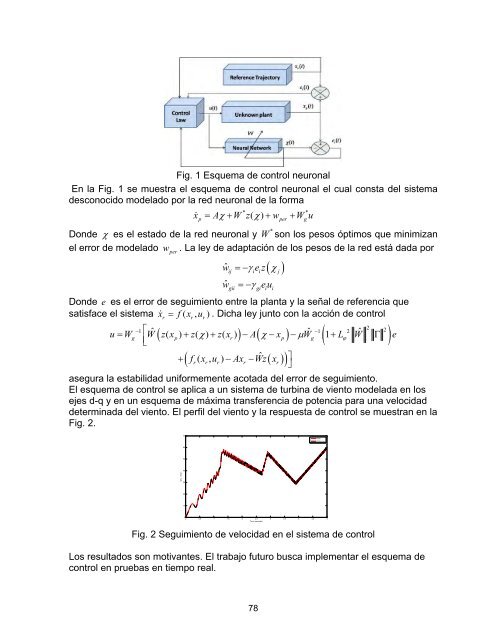
Fig. 1 Esquema <strong>de</strong> control neuronal<br />
En la Fig. 1 se muestra el esquema <strong>de</strong> control neuronal el cual consta <strong>de</strong>l sistema<br />
<strong>de</strong>sconocido mo<strong>de</strong>lado por la red neuronal <strong>de</strong> la forma<br />
* *<br />
x&<br />
= Aχ<br />
+ W z( χ)<br />
+ w + W u<br />
p per g<br />
*<br />
Don<strong>de</strong> χ es el estado <strong>de</strong> la red neuronal y W son los pesos óptimos que minimizan<br />
el error <strong>de</strong> mo<strong>de</strong>lado . La ley <strong>de</strong> adaptación <strong>de</strong> los pesos <strong>de</strong> la red está dada por<br />
w per<br />
wˆ<br />
wˆ<br />
=−γ<br />
ez<br />
=−γ<br />
eu<br />
( χ )<br />
ij i i j<br />
gii gi i i<br />
Don<strong>de</strong> e es el error <strong>de</strong> seguimiento entre la planta y la señal <strong>de</strong> referencia que<br />
satisface el sistema x&<br />
r<br />
= f ( xr, ur)<br />
. Dicha ley junto con la acción <strong>de</strong> control<br />
2<br />
−1 1<br />
2<br />
u W<br />
⎡ ˆ ( ) ( ) ˆ −<br />
2<br />
=<br />
g<br />
W z( xp) + z( χ) + z( xr) − A χ −xp − µ Wg<br />
( 1+<br />
L Wˆ ϕ<br />
Γ ) e<br />
⎢⎣<br />
+ ( f ( , ) ˆ<br />
r<br />
xr ur −Axr −Wz( xr)<br />
) ⎤<br />
⎦<br />
asegura la estabilidad uniformemente acotada <strong>de</strong>l error <strong>de</strong> seguimiento.<br />
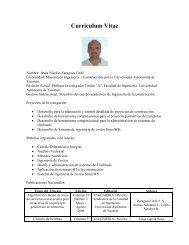
El esquema <strong>de</strong> control se aplica a un sistema <strong>de</strong> turbina <strong>de</strong> viento mo<strong>de</strong>lada en los<br />
ejes d-q y en un esquema <strong>de</strong> máxima transferencia <strong>de</strong> potencia para una velocidad<br />
<strong>de</strong>terminada <strong>de</strong>l viento. El perfil <strong>de</strong>l viento y la respuesta <strong>de</strong> control se muestran en la<br />
Fig. 2.<br />
70<br />
Wm<br />
Reference<br />
60<br />
50<br />
40<br />
Wm, Wref<br />
30<br />
20<br />
10<br />
0<br />
0 0.5 1 1.5 2 2.5 3 3.5 4 4.5 5<br />
Time (seconds)<br />
Fig. 2 Seguimiento <strong>de</strong> velocidad en el sistema <strong>de</strong> control<br />
Los resultados son motivantes. El trabajo futuro busca implementar el esquema <strong>de</strong><br />
control en pruebas en tiempo real.<br />
78