Approximations multiéchelles - Laboratoire Jacques-Louis Lions ...

1.0
0.5
initiale
recons
0.0
0.0 0.5 1.0
1.0
0.5
initiale
mr
++
+ +
++
++
++
++
++
++
+++++ ++++
++
++
++
++
++
++
++
++
+ +
++ ++++++++++++ + + +
+ ++ +++++
+ ++ +++++++++
0.0
0.0 0.5 1.0
10
8
6
4
2
+ +
+ + + +
+++++++++++++++++++++ +++++++++++
+++++++++++
+ +
+ +
+ + + +
0
0.0 0.5 1.0
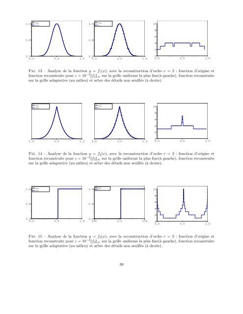
Fig. 13 – Analyse de la fonction y = f1(x), avec la reconstruction d’ordre r = 2 : fonction d’origine et
fonction reconstruite pour ε = 10 −3 |f1 |∞ sur la grille uniforme la plus fine(à gauche), fonction reconstruite
sur la grille adaptative (au milieu) et arbre des détails non seuillés (à droite).
initiale
recons
0.0 0.5 1.0
initiale
mr
++
++
+ + + ++ + + + ++ ++ +++++++++++++
++
++
++ ++
++
++
++ ++ + ++
++
++
++
++
++
++
++
+++++++++++
++
++
+ + + + +
+
0.0 0.5 1.0
10
8
6
4
2
+ + + + + + + + + +
+
+
++ ++
++++++++++++++
++++++++++++++
+
+ + + + + + + + +
0
0.0 0.5 1.0
Fig. 14 – Analyse de la fonction y = f2(x), avec la reconstruction d’ordre r = 2 : fonction d’origine et
fonction reconstruite pour ε = 10 −3 |f2 |∞ sur la grille uniforme la plus fine(à gauche), fonction reconstruite
sur la grille adaptative (au milieu) et arbre des détails non seuillés (à droite).
1.0
0.5
initiale
recons
0.0
0.0 0.5 1.0
1.0
0.5
initiale
mr
+
+++ + + + + + + +++
+ + + + +++++
+++ +
0.0
0.0 0.5 1.0
+
+
+
+
+
++
++
+ +
+ +
+ + +
+ +
++ +++
+ +
+
+
+
+
+ +
++ +++
+ + +
+ + +
+ +
+ +
0
0.0 0.5 1.0
Fig. 15 – Analyse de la fonction y = f3(x), avec la reconstruction d’ordre r = 2 : fonction d’origine et
fonction reconstruite pour ε = 10 −3 |f3 |∞ sur la grille uniforme la plus fine(à gauche), fonction reconstruite
sur la grille adaptative (au milieu) et arbre des détails non seuillés (à droite).
30
10
8
6
4
2
++
+ +
+
+
+
+
+
++