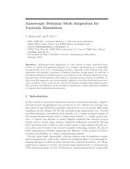
Fig. 27 – Solution adaptative au début de la simulation. Fig. 28 – Grille adaptative à la fin de la simulation. Fig. 29 – Solution adaptative à la fin de la simulation. 50
S ℓ i,j : A(T )p ℓ i,j = A(T )u, if T ∈ V ℓ i,j. (110) The reconstructed solution is defined as the mean value of this polynomial on the subtriangle T ℓ+1 i,j containing the given vertices Sℓ i,j (as shown on figure 30). ũ ℓ+1 i,j = A(T ℓ+1 i,j )pℓ i,j for j = 1, . . . , 3. (111) The mean value on the central subtriangle is computed by imposing conservation of the total sum on T ℓ i , see (34). The case M = 1 (i.e. second order accurate reconstruction) was numerically experimented in [37], together with other strategies to select p ∈ Π1. We shall see below that a straightforward selection of p that mimics the 1D construction fails to provide a stable reconstruction in the sense that the limit function is not even in L1 , and we shall propose a modified prediction operator which overcomes this drawback. We denote by T ℓ 0 the current triangle and T ℓ i , i = 1, 2, 3, the three triangles that share an edge with T ℓ 0. Their numbering is such that the vertex Sℓ 0,j of T ℓ 0 does not belong to T ℓ j . Then the most natural choice for . A similar construction is done p0,3 seems to be by imposing (110) on T ℓ 0 and the two neighbors T ℓ 1 and T ℓ 2 for p0,1 and p0,2. Writing p ℓ 0,3(x, y) = a ℓ 0,3x + b ℓ 0,3y + c ℓ 0,3, (112) and using the fact that for a polynomial of degree 1 one has A(T ℓ k )pℓ0,3 = pℓ0,3 (xℓ k , yℓ k ), we obtain the three equations a ℓ 0,3xℓk + bℓ0,3yℓ k + cℓ0,3 = ūℓk , (113) ℓ x for k ∈ {0, 1, 2}. The coefficients a0,3 and b0,3 solve a 2 × 2 linear system whose matrix 1 − xℓ 0 yℓ 1 − yℓ 0 x ℓ 2 − xℓ 0 is non singular if the two centroids of T ℓ 1 and T ℓ 2 are not aligned with the current centroid Gℓ 0 y ℓ 2 − yℓ 0 , which is the case for uniform triangulations. The last coefficient c0,3 is computed by (113). A particular feature of this decomposition is that, for uniform triangulations, the centroid of the triangle T ℓ+1 0,3 is also the midpoint of the segment between the centroids of the triangles T ℓ 1 and T ℓ 2. Therefore any plane containing both points 1 , yℓ+1 0,3 , 2 (ūℓ1 + ūℓ2 )) whatever be the value of p(xℓ0 , yℓ 0 ). does not depend on the value of the (xℓ 1 , yℓ 1 , ū1) and (xℓ 2 , yℓ 2 , ū2) also contains the point (x ℓ+1 0,3 In other words the interpolated value on non central subtriangles of T ℓ 0 function on T ℓ 0 : ũ ℓ+1 0,3 = 1 2 (ūℓ 1 + ū ℓ 2). (114) This remark enables to show on a simple example that this scheme is not stable. We consider the case of a piecewise constant function equal to one on a triangle T 0 0 and to zero everywhere else. After n iterations of the subdivision scheme the reconstructed function takes the value 4 n on the center triangle of the n th level which clearly means that the limit function is not bounded (and not even in L 1 since it features a Dirac at the origin). We have not yet analyzed the higher degree reconstructions from this point of view, but they present anyway the other drawback of requiring much larger stencils to compute the local reconstruction polynomials. We adopt therefore an alternate solution consisting (again in the case of uniform decomposition) in the following reconstruction scheme on four triangles : ⎧ ⎪⎨ ⎪⎩ ũ ℓ+1 0,0 = ūℓ 0 , ũ ℓ+1 0,1 = ūℓ 0 + (ūℓ 2 + ūℓ 3 − 2ūℓ 1 )/6, ũ ℓ+1 0,2 = ūℓ 0 + (ū ℓ 1 + ū ℓ 3 − 2ū ℓ 2)/6, ũ ℓ+1 0,3 = ūℓ 0 + (ū ℓ 1 + ū ℓ 2 − 2ū ℓ 3)/6. Although not based on a polynomial selection process, this reconstruction is still exact for polynomials of degree one and thus second order accurate. Moreover, it is stable, in the sense that the limit function has C t smoothness for all t < 1. 51 (115)