- Page 1 and 2:
U N I R A P E D T T E M D S E N TA
- Page 3:
C O L A N IO T A N U N C I EA .S. D
- Page 6 and 7:
This report was prepared under cont
- Page 8 and 9:
Table of Contents Acronyms and Abbr
- Page 10 and 11:
C.1 Journal Publications ..........
- Page 12 and 13:
Figure 18. Encounter rate models bu
- Page 14 and 15:
List of Tables Table 1. Summary of
- Page 16 and 17:
Appendix B, Table B-6. Summary of m
- Page 18 and 19:
Acknowledgements This project was f
- Page 20 and 21:
of these choices as possible and us
- Page 22 and 23:
Although our models include most of
- Page 24 and 25:
2.0 Background The Navy and other m
- Page 26 and 27:
comparison is based on a separate s
- Page 28 and 29:
Figure 1. Transects (green lines) s
- Page 30 and 31:
used to evaluate the ability of sum
- Page 32 and 33:
3.1.5 Mid-trophic Sampling with Net
- Page 34 and 35:
variable. Interpolated maps of the
- Page 36 and 37:
Table 2. Variogram model results. A
- Page 38 and 39:
“number of individuals” as the
- Page 40 and 41:
Encounter Rate and Group Size Model
- Page 42 and 43:
were built separately for each of t
- Page 44 and 45:
Expanding models to the entire U.S.
- Page 46 and 47:
Table 4. Summary of the weighted ef
- Page 48 and 49:
Consistent with Barlow and Forney (
- Page 50 and 51:
incorporation of geographic coordin
- Page 52 and 53:
overwhelming majority of “Bryde
- Page 54 and 55:
the genera Ziphius and Mesoplodon.
- Page 56 and 57:
Table 7. Geographically stratified
- Page 58 and 59:
above, and the data themselves, are
- Page 60 and 61:
(hereafter “summer”). SWFSC has
- Page 62 and 63:
avoid these problems, we decided to
- Page 64 and 65:
Figure 9. Thermocline depth (m) obs
- Page 66 and 67:
Attempts to adjust search parameter
- Page 68 and 69:
CAMMS 1991 PODS 1993 ORCAWALE 1996
- Page 70 and 71:
4.2 Modeling Framework : GLM and GA
- Page 72 and 73:
4.2.4 Conclusions Regardings Modeli
- Page 74 and 75:
Table 10 cont. Comparison of the si
- Page 76 and 77:
Table 11 cont. Comparison of the si
- Page 78 and 79:
Figure 15. The transect lines used
- Page 80 and 81:
A) Striped dolphin 10 km B) Short-b
- Page 82 and 83:
dependent. For example, the number
- Page 84 and 85:
Figure 19. Predicted average densit
- Page 86 and 87: ecosystem, eastern spinner dolphins
- Page 88 and 89: Table 13. Variables selected for mo
- Page 90 and 91: Table 14. Starting and final AIC va
- Page 92 and 93: Table 17. Ratios of observed to pre
- Page 94 and 95: species represented in the acoustic
- Page 96 and 97: 0.29 (Risso’s dolphin) to 3.20 (n
- Page 98 and 99: Figure 25. Sample 2005 validation p
- Page 100 and 101: Table 18. (continued) 1991 1993 Nor
- Page 102 and 103: Blue whales had the greatest deviat
- Page 104 and 105: Table 20. Abundance (number of anim
- Page 106 and 107: Table 22. Proportion of deviance ex
- Page 108 and 109: Figure 27. Average density (AveDens
- Page 110 and 111: Table 23. Effective degrees of free
- Page 112 and 113: We attempted to build encounter rat
- Page 114 and 115: 5.0 Conclusion The field of predict
- Page 116 and 117: 6.0 Transition Plan The models of c
- Page 118 and 119: needed to ensure that the SDSS rema
- Page 120 and 121: Administrative Report LJ-07-02. NOA
- Page 122 and 123: Forney KA, Barlow J (1993) Prelimin
- Page 124 and 125: Redfern JV, Barlow J, Ballance LT,
- Page 126 and 127: Appendix A: Detailed Model Results
- Page 128 and 129: Table A-1 (continued) Blue whale 19
- Page 130 and 131: Figure A-1a. Striped dolphin 108
- Page 132 and 133: Figure A-1c. Risso’s dolphin 110
- Page 134 and 135: Figure A-1e. Northern right whale d
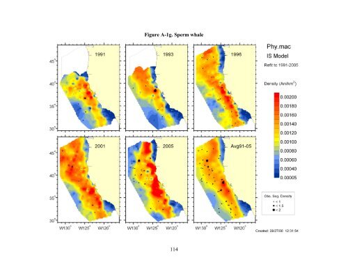
- Page 138 and 139: Figure A-1i. Blue whale 116
- Page 140 and 141: Figure A-1k. Baird’s beaked whale
- Page 142 and 143: Figure A-2. Predicted average densi
- Page 144 and 145: Figure A-2b. Short-beaked common do
- Page 146 and 147: Figure A-2d. Pacific white-sided do
- Page 148 and 149: Figure A-2f. Dall’s porpoise 126
- Page 150 and 151: Figure A-2h. Fin whale 128
- Page 152 and 153: Figure A-2j. Humpback whale 130
- Page 154 and 155: Figure A-2l. Small beaked whales 13
- Page 156 and 157: Table B-2. Summary of model validat
- Page 158 and 159: Table B-3. Summary of model validat
- Page 160 and 161: Table B-4. Summary of model validat
- Page 162 and 163: Table B-5. Summary of model validat
- Page 164 and 165: Table B-6. Summary of model validat
- Page 166 and 167: Table B-7. Summary of model validat
- Page 168 and 169: Table B-8. Summary of model validat
- Page 170 and 171: Table B-9. Summary of model validat
- Page 172 and 173: Table B-10. Summary of model valida
- Page 174 and 175: Table B-11. Summary of model valida
- Page 176 and 177: Table B-12. Summary of model valida
- Page 178 and 179: Table B-13. Summary of model valida
- Page 180 and 181: Table B-14. Summary of model valida
- Page 182 and 183: Table B-15. Summary of model valida
- Page 184 and 185: Figure B-1. Predicted yearly and av
- Page 186 and 187:
Figure B-1. b) Eastern spinner dolp
- Page 188 and 189:
Figure B-1. c) Whitebelly spinner d
- Page 190 and 191:
Figure B-1. d) Striped dolphin 168
- Page 192 and 193:
Figure B-1. e) Rough-toothed dolphi
- Page 194 and 195:
Figure B-1. f) Short-beaked common
- Page 196 and 197:
Figure B-1. g) Bottlenose dolphin 1
- Page 198 and 199:
Figure B-1. h) Risso’s dolphin 17
- Page 200 and 201:
Figure B-1. i) Cuvier’s beaked wh
- Page 202 and 203:
Figure B-1. j) Blue whale 180
- Page 204 and 205:
Figure B-1. k) Bryde’s whale 182
- Page 206 and 207:
Figure B-1. l) Short-finned pilot w
- Page 208 and 209:
Figure B-1. m) Dwarf sperm whale 18
- Page 210 and 211:
Figure B-1. n) Mesoplodon beaked wh
- Page 212 and 213:
Figure B-1. o) Small beaked whales
- Page 214 and 215:
Figure B-2. Predicted average densi
- Page 216 and 217:
Figure B-2. (cont.) c) Whitebelly s
- Page 218 and 219:
Figure B-2. (cont.) g) Bottlenose d
- Page 220 and 221:
Figure B-2. (cont.) k) Bryde’s wh
- Page 222 and 223:
Figure B-2. (cont.) o) Small beaked
- Page 224 and 225:
Ferguson MC (2005) Cetacean Populat
- Page 226 and 227:
Barlow J, Kahru M, Mitchell BG (In
- Page 228 and 229:
Memorandum NMFS-SWFSC-374, U.S. Dep