Linear Programming Lecture Notes - Penn State Personal Web Server

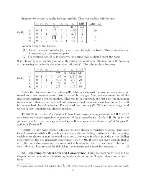
Suppose we choose s4 as the leaving variable. Then our tableau will become:
⎡
⎤
z x1 x2 s1 s2 s3 s4 RHS MRT (s1)
z ⎢ 1 0 0 −14/5 0 0 44/5 544 ⎥
x1 ⎢
(5.47) ⎢ 0 1 0 4/5 0 0 −4/5 16 ⎥ 20
x2 ⎢
0 0 1 −7/5 0 0 12/5 72 ⎥ −
s2 ⎣ 0 0 0 2 1 0 −4 0 ⎦ 0
s3 0 0 0 −4/5 0 1 4/5 19 −
We now observe two things:
(1) One of the basic variables (s2) is zero, even though it is basic. This is the indicator
of degeneracy at an extreme point.
(2) The reduced cost of s1 is negative, indicating that s1 should enter the basis.
If we choose s1 as an entering variable, then using the minimum ratio test, we will choose s2
as the leaving variable (by the minimum ratio test) 2 . Then the tableau becomes:
(5.48)
z
x1
x2
s1
⎡
z
⎢ 1
⎢ 0
⎢ 0
⎣ 0
x1
0
1
0
0
x2
0
0
1
0
s1
0
0
0
1
s2
7/5
−2/5
7/10
1/2
s3
0
0
0
0
s4
16/5
4/5
−2/5
−2
⎤
RHS
544 ⎥
16 ⎥
72 ⎥
0 ⎦
0 0 0 0 2/5 1 −4/5 19
s3
Notice the objective function value cBB −1 b has not changed, because we really have not
moved to a new extreme point. We have simply changed from one representation of the
degenerate extreme point to another. This was to be expected, the fact that the minimum
ratio was zero showed that we could not increase s1 and maintain feasibility. As such s1 = 0
in the new basic feasible solution. The reduced cost vector cBB −1 N − cN has changed and
we could now terminate the simplex method.
Theorem 5.16. Consider Problem P (our linear programming problem). Let B ∈ R m×m
be a basis matrix corresponding to some set of basic variables xB. Let b = B −1 b. If bj = 0
for some j = 1, . . . , m, then xB = b and xN = 0 is a degenerate extreme point of the feasible
region of Problem P .
Proof. At any basic feasible solutions we have chosen m variables as basic. This basic
feasible solution satisfies BxB = b and thus provides m binding constraints. The remaining
variables are chosen as non-basic and set to zero, thus xN = 0, which provides n−m binding
constraints on the non-negativity constraints (i.e., x ≥ 0). If there is a basic variable that is
zero, then an extra non-negativity constraint is binding at that extreme point. Thus n + 1
constraints are binding and, by definition, the extreme point must be degenerate.
7.1. The Simplex Algorithm and Convergence. Using the work we’ve done in this
chapter, we can now state the following implementation of the Simplex algorithm in matrix
form.
2 The minimum ratio test still applies when bj = 0. In this case, we will remain at the same extreme point.
88