Linear Programming Lecture Notes - Penn State Personal Web Server

More documents

Recommendations

Info

point in Y we know that at most m elements of the vector x are non-zero and therefore, every extreme point in Y corresponds to an extreme point of the original problem P . Since Problem P has a finite solution, it follows that the optimal solution to problem P occurs at some point in Y, by Theorem 5.1. Furthermore the value of the objective function for Problem P is precisely the same as the value of the objective function of Problem PM for each point in Y because xa = 0. Define: (6.22) z min P = min y∈Y {cT x : y = [x xa] T } At each extreme point in Ya, the value of the objective function of Problem PM is a function of the value of M, which we are free to choose. Therefore, choose M so that: (6.23) max{c y∈Ya T x − Me T xa : y = [x xa] T } < z min P Such a value exists for M since there are only a finite number of extreme points in Y. Our choice of M ensures that the optimal solution to PM occurs at an extreme point where xa = 0 and the x component of y is the solution to Problem P . Remark 6.10. Another way to look at the proof of this theorem is to think of defining M in such a way so that at any extreme point where xa = 0, the objective function can always be made larger by moving to any extreme point that is feasible to Problem P . Thus the simplex algorithm will move among the extreme points seeking to leave those that are not feasible to Problem P because they are less desirable. Theorem 6.11. Suppose Problem P is infeasible. Then there is no value of M that will drive the all the artificial variables from the basis of Problem PM. Proof. If such an M existed, then xa = 0 and the resulting values of x represents a feasible solution to Problem P , which contradicts our assumption that Problem P was infeasible. Remark 6.12. The Big-M method is not particularly effective for solving real-world problems. The introduction of a set of variables with large coefficients (M) can lead to round-off errors in the execution of the simplex algorithm. (Remember, computers can only manipulate numbers in binary, which means that all floating point numbers are restricted in their precision to the machine precision of the underlying system OS. This is generally given in terms of the largest amount of memory that can be addressed in bits. This has led, in recent times, to operating system manufacturers selling their OS’s as “32 bit” or “64 bit.” When solving real-world problems, these issue can become a real factor with which to contend. Another issue is we have no way of telling how large M should be without knowing that Problem P is feasible, which is precisely what we want the Big-M method to tell us! The general rule of thumb provided earlier will suffice. 100
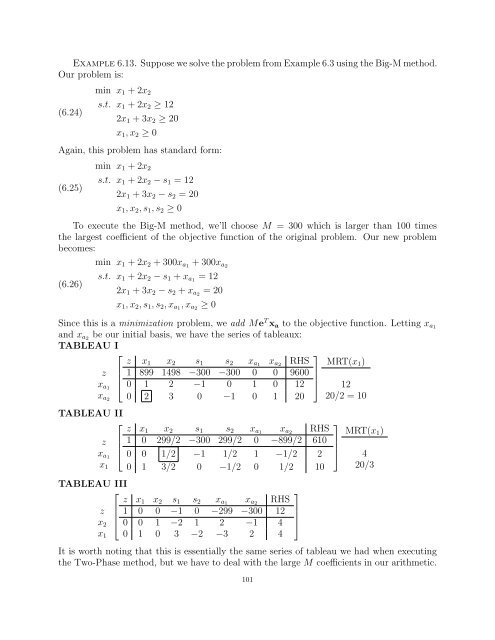
Example 6.13. Suppose we solve the problem from Example 6.3 using the Big-M method. Our problem is: (6.24) min x1 + 2x2 s.t. x1 + 2x2 ≥ 12 2x1 + 3x2 ≥ 20 x1, x2 ≥ 0 Again, this problem has standard form: (6.25) min x1 + 2x2 s.t. x1 + 2x2 − s1 = 12 2x1 + 3x2 − s2 = 20 x1, x2, s1, s2 ≥ 0 To execute the Big-M method, we’ll choose M = 300 which is larger than 100 times the largest coefficient of the objective function of the original problem. Our new problem becomes: min x1 + 2x2 + 300xa1 + 300xa2 s.t. x1 + 2x2 − s1 + xa1 = 12 (6.26) 2x1 + 3x2 − s2 + xa2 = 20 x1, x2, s1, s2, xa1, xa2 ≥ 0 Since this is a minimization problem, we add Me T xa to the objective function. Letting xa1 and xa2 be our initial basis, we have the series of tableaux: TABLEAU I ⎡ z xa1 xa2 ⎢ ⎣ TABLEAU II ⎡ z xa1 x1 ⎢ ⎣ z x1 x2 s1 s2 xa1 xa2 RHS 1 899 1498 −300 −300 0 0 9600 0 1 2 −1 0 1 0 12 0 2 3 0 −1 0 1 20 z x1 x2 s1 s2 xa1 xa2 RHS 1 0 299/2 −300 299/2 0 −899/2 610 0 0 1/2 −1 1/2 1 −1/2 2 0 1 3/2 0 −1/2 0 1/2 10 TABLEAU III ⎡ z z ⎢ 1 x2 ⎣ 0 x1 0 0 x2 0 1 s1 −1 −2 s2 0 1 xa1 −299 2 xa2 −300 −1 RHS 12 4 0 1 0 3 −2 −3 2 4 x1 ⎤ ⎥ ⎦ ⎤ ⎥ ⎦ MRT(x1) 12 20/2 = 10 ⎤ ⎥ ⎦ MRT(x1) 4 20/3 It is worth noting that this is essentially the same series of tableau we had when executing the Two-Phase method, but we have to deal with the large M coefficients in our arithmetic. 101
Page 1:
Linear Programming: Penn State Math
Page 4 and 5:
8. Caratheodory Characterization Th
Page 7 and 8:
List of Figures 1.1 Goat pen with u
Page 9 and 10:
4.6 Convex Direction: Clearly every
Page 11:
Preface Stop! Stop right now! This
Page 14 and 15:
x Goat Pen Figure 1.1. Goat pen wit
Page 16 and 17:
We have formulated the general maxi
Page 18 and 19:
Figure 1.3. Contour Plot of z = x 2
Page 20 and 21:
Figure 1.5. A Level Curve Plot with
Page 22 and 23:
and thus our vector is v = (x1 −
Page 24 and 25:
Figure 1.7. Gradients of the Bindin
Page 26 and 27:
finishing toys and 120 hours per we
Page 28 and 29:
2. Graphically Solving Linear Progr
Page 30 and 31:
S r x 0 Br( x0) Figure 2.2. A Bound
Page 32 and 33:
S Every point on this line is an al
Page 34:
6. Problems with Unbounded Feasible
Page 37:
to “prove” your example works.
Page 40 and 41:
Definition 3.6 (Matrix Transpose).
Page 42 and 43:
3. Matrices and Linear Programming
Page 44 and 45:
Remark 3.16. We can deal with const
Page 46 and 47:
Theorem 3.20. Each elementary row o
Page 48 and 49:
Gauss-Jordan Elimination Computing
Page 50 and 51:
and right hand side vector b = [7,
Page 52 and 53:
Gauss-Jordan elimination to solve t
Page 54 and 55:
which clearly has a solution for al
Page 56 and 57:
which is a contradiction. Case 2: S
Page 58 and 59:
Definition 3.46 (Basic Variables).
Page 60 and 61:
This leads to the following linear
Page 62 and 63: This is not in a form Matlab likes,
Page 64 and 65: Example 4.5. Figure 4.1 illustrates
Page 66 and 67: Figure 4.3. A hyperplane in 3 dimen
Page 68 and 69: 4. Rays and Directions Recall the d
Page 70 and 71: for all λ > 0. This can only be tr
Page 72 and 73: Theorem 4.31. Let P ⊆ R n be a po
Page 74 and 75: Figure 4.9. A Polyhedral Set: This
Page 76 and 77: Figure 4.10. Visualization of the s
Page 78 and 79: It is clear that P is bounded. In f
Page 80 and 81: x1 x5 x2 x λx2 +(1− λ)x3 x4 x3
Page 82 and 83: If there is some i such that c T di
Page 84 and 85: Consider now the fact xj = 0 for al
Page 86 and 87: Example 5.9. Consider the Toy Maker
Page 88 and 89: using this information, we can comp
Page 90 and 91: Figure 5.1. The Simplex Algorithm:
Page 92 and 93: Using this information, we can see
Page 94 and 95: Based on this information, we can c
Page 96 and 97: Using the rule you developed in Exe
Page 98 and 99: Exercise 52. Consider the diet prob
Page 100 and 101: Suppose we choose s4 as the leaving
Page 103 and 104: CHAPTER 6 Simplex Initialization In
Page 105 and 106: A basic feasible solution for our a
Page 107 and 108: variables. This is because we start
Page 109 and 110: To remove the artificial variables
Page 111: Remark 6.6. In the case of a minimi
Page 115 and 116: That is, s1 = −12 and s2 = −20
Page 117 and 118: The complete problem describing McL
Page 119: * data section */ data; set DAY :=
Page 122 and 123: This leads to a vector of reduced c
Page 124 and 125: 2.1. Lexicographic Minimum Ratio Te
Page 126 and 127: Proof. The initial basis Im yieds a
Page 128 and 129: for i = 1, . . . , n. Then we have:
Page 130 and 131: Revised Simplex Algorithm (1) Ident
Page 132 and 133: simplex tableau). We obtain: z1 −
Page 134 and 135: Proof. We can prove Farkas’ Lemma
Page 136 and 137: A1· Half-space cy > 0 A2· c Am·
Page 138 and 139: 3. The Karush-Kuhn-Tucker Condition
Page 140 and 141: Remark 8.9. The expressions: ∗ A
Page 142 and 143: (x ∗ 1,x ∗ 2) = (16, 72) 3x1 +
Page 144 and 145: Since w1, w2 ≥ 0, we know that w
Page 146 and 147: Example 8.13. Consider the followin
Page 148 and 149: Figure 8.5. This figure illustrates
Page 150 and 151: (9.4) Proof. Rewrite Problem D as:
Page 152 and 153: This vector will be related to c in
Page 154 and 155: 3. Strong Duality Lemma 9.7. Proble
Page 156 and 157: Likewise beginning with the KKT con
Page 158 and 159: egions are polyhedral sets 1 . Cert
Page 160 and 161: Figure 9.2. The simplex algorithm b
Page 162 and 163:
If a selfish profit maximizer wishe
Page 164 and 165:
Recall the optimal full tableau for
Page 166 and 167:
For the sake of space, we will prov
Page 168 and 169:
We can choose either s1 or s2 as a
show all

Linear Programming Lecture Notes - Penn State Personal Web Server

Create successful ePaper yourself

Delete template?

Save as template?