

Linear Programming Lecture Notes - Penn State Personal Web Server
Linear Programming Lecture Notes - Penn State Personal Web Server
Linear Programming Lecture Notes - Penn State Personal Web Server

You also want an ePaper? Increase the reach of your titles
YUMPU automatically turns print PDFs into web optimized ePapers that Google loves.
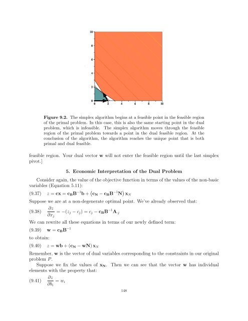
Figure 9.2. The simplex algorithm begins at a feasible point in the feasible region<br />
of the primal problem. In this case, this is also the same starting point in the dual<br />
problem, which is infeasible. The simplex algorithm moves through the feasible<br />
region of the primal problem towards a point in the dual feasible region. At the<br />
conclusion of the algorithm, the algorithm reaches the unique point that is both<br />
primal and dual feasible.<br />
feasible region. Your dual vector w will not enter the feasible region until the last simplex<br />
pivot.]<br />
5. Economic Interpretation of the Dual Problem<br />
Consider again, the value of the objective function in terms of the values of the non-basic<br />
variables (Equation 5.11):<br />
(9.37) z = cx = cBB −1 b + cN − cBB −1 N xN<br />
Suppose we are at a non-degenerate optimal point. We’ve already observed that:<br />
∂z<br />
(9.38) = −(zj − cj) = cj − cBB<br />
∂xj<br />
−1 A·j<br />
We can rewrite all these equations in terms of our newly defined term:<br />
(9.39) w = cBB −1<br />
to obtain:<br />
(9.40) z = wb + (cN − wN) xN<br />
Remember, w is the vector of dual variables corresponding to the constraints in our original<br />
problem P .<br />
Suppose we fix the values of xN.<br />
elements with the property that:<br />
Then we can see that the vector w has individual<br />
(9.41)<br />
∂z<br />
∂bi<br />
= wi<br />
148


