Linear Programming Lecture Notes - Penn State Personal Web Server

More documents

Recommendations

Info

S Every point on this line is an alternative optimal solution. Figure 2.3. An example of infinitely many alternative optimal solutions in a linear programming problem. The level curves for z(x1, x2) = 18x1 + 6x2 are parallel to one face of the polygon boundary of the feasible region. Moreover, this side contains the points of greatest value for z(x1, x2) inside the feasible region. Any combination of (x1, x2) on the line 3x1+x2 = 120 for x1 ∈ [16, 35] will provide the largest possible value z(x1, x2) can take in the feasible region S. the new problem and obtain a description for the set of alternative optimal solutions. [Hint: Just as in the example, x1 will be bound between two value corresponding to a side of the polygon. Find those values and the constraint that is binding. This will provide you with a description of the form for any x ∗ 1 ∈ [a, b] and x ∗ 2 is chosen so that cx ∗ 1 + dx ∗ 2 = v, the point (x ∗ 1, x ∗ 2) is an alternative optimal solution to the problem. Now you fill in values for a, b, c, d and v.] 5. Problems with No Solution Recall for any mathematical programming problem, the feasible set or region is simply a subset of R n . If this region is empty, then there is no solution to the mathematical programming problem and the problem is said to be over constrained. We illustrate this case for linear programming problems with the following example. Example 2.8. Consider the following linear programming problem: ⎧ max z(x1, x2) = 3x1 + 2x2 ⎪⎨ s.t. (2.11) ⎪⎩ 1 40 x1 + 1 60 x2 ≤ 1 1 50 x1 + 1 50 x2 ≤ 1 x1 ≥ 30 x2 ≥ 20 20
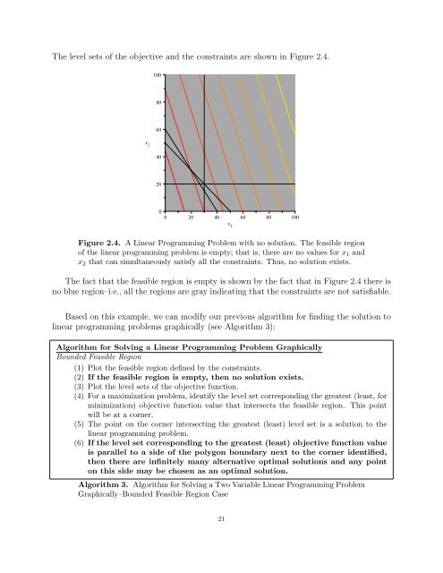
The level sets of the objective and the constraints are shown in Figure 2.4. Figure 2.4. A Linear Programming Problem with no solution. The feasible region of the linear programming problem is empty; that is, there are no values for x1 and x2 that can simultaneously satisfy all the constraints. Thus, no solution exists. The fact that the feasible region is empty is shown by the fact that in Figure 2.4 there is no blue region–i.e., all the regions are gray indicating that the constraints are not satisfiable. Based on this example, we can modify our previous algorithm for finding the solution to linear programming problems graphically (see Algorithm 3): Algorithm for Solving a Linear Programming Problem Graphically Bounded Feasible Region (1) Plot the feasible region defined by the constraints. (2) If the feasible region is empty, then no solution exists. (3) Plot the level sets of the objective function. (4) For a maximization problem, identify the level set corresponding the greatest (least, for minimization) objective function value that intersects the feasible region. This point will be at a corner. (5) The point on the corner intersecting the greatest (least) level set is a solution to the linear programming problem. (6) If the level set corresponding to the greatest (least) objective function value is parallel to a side of the polygon boundary next to the corner identified, then there are infinitely many alternative optimal solutions and any point on this side may be chosen as an optimal solution. Algorithm 3. Algorithm for Solving a Two Variable Linear Programming Problem Graphically–Bounded Feasible Region Case 21
Page 1: Linear Programming: Penn State Math
Page 4 and 5: 8. Caratheodory Characterization Th
Page 7 and 8: List of Figures 1.1 Goat pen with u
Page 9 and 10: 4.6 Convex Direction: Clearly every
Page 11: Preface Stop! Stop right now! This
Page 14 and 15: x Goat Pen Figure 1.1. Goat pen wit
Page 16 and 17: We have formulated the general maxi
Page 18 and 19: Figure 1.3. Contour Plot of z = x 2
Page 20 and 21: Figure 1.5. A Level Curve Plot with
Page 22 and 23: and thus our vector is v = (x1 −
Page 24 and 25: Figure 1.7. Gradients of the Bindin
Page 26 and 27: finishing toys and 120 hours per we
Page 28 and 29: 2. Graphically Solving Linear Progr
Page 30 and 31: S r x 0 Br( x0) Figure 2.2. A Bound
Page 34: 6. Problems with Unbounded Feasible
Page 37: to “prove” your example works.
Page 40 and 41: Definition 3.6 (Matrix Transpose).
Page 42 and 43: 3. Matrices and Linear Programming
Page 44 and 45: Remark 3.16. We can deal with const
Page 46 and 47: Theorem 3.20. Each elementary row o
Page 48 and 49: Gauss-Jordan Elimination Computing
Page 50 and 51: and right hand side vector b = [7,
Page 52 and 53: Gauss-Jordan elimination to solve t
Page 54 and 55: which clearly has a solution for al
Page 56 and 57: which is a contradiction. Case 2: S
Page 58 and 59: Definition 3.46 (Basic Variables).
Page 60 and 61: This leads to the following linear
Page 62 and 63: This is not in a form Matlab likes,
Page 64 and 65: Example 4.5. Figure 4.1 illustrates
Page 66 and 67: Figure 4.3. A hyperplane in 3 dimen
Page 68 and 69: 4. Rays and Directions Recall the d
Page 70 and 71: for all λ > 0. This can only be tr
Page 72 and 73: Theorem 4.31. Let P ⊆ R n be a po
Page 74 and 75: Figure 4.9. A Polyhedral Set: This
Page 76 and 77: Figure 4.10. Visualization of the s
Page 78 and 79: It is clear that P is bounded. In f
Page 80 and 81: x1 x5 x2 x λx2 +(1− λ)x3 x4 x3
Page 82 and 83:
If there is some i such that c T di
Page 84 and 85:
Consider now the fact xj = 0 for al
Page 86 and 87:
Example 5.9. Consider the Toy Maker
Page 88 and 89:
using this information, we can comp
Page 90 and 91:
Figure 5.1. The Simplex Algorithm:
Page 92 and 93:
Using this information, we can see
Page 94 and 95:
Based on this information, we can c
Page 96 and 97:
Using the rule you developed in Exe
Page 98 and 99:
Exercise 52. Consider the diet prob
Page 100 and 101:
Suppose we choose s4 as the leaving
Page 103 and 104:
CHAPTER 6 Simplex Initialization In
Page 105 and 106:
A basic feasible solution for our a
Page 107 and 108:
variables. This is because we start
Page 109 and 110:
To remove the artificial variables
Page 111 and 112:
Remark 6.6. In the case of a minimi
Page 113 and 114:
Example 6.13. Suppose we solve the
Page 115 and 116:
That is, s1 = −12 and s2 = −20
Page 117 and 118:
The complete problem describing McL
Page 119:
* data section */ data; set DAY :=
Page 122 and 123:
This leads to a vector of reduced c
Page 124 and 125:
2.1. Lexicographic Minimum Ratio Te
Page 126 and 127:
Proof. The initial basis Im yieds a
Page 128 and 129:
for i = 1, . . . , n. Then we have:
Page 130 and 131:
Revised Simplex Algorithm (1) Ident
Page 132 and 133:
simplex tableau). We obtain: z1 −
Page 134 and 135:
Proof. We can prove Farkas’ Lemma
Page 136 and 137:
A1· Half-space cy > 0 A2· c Am·
Page 138 and 139:
3. The Karush-Kuhn-Tucker Condition
Page 140 and 141:
Remark 8.9. The expressions: ∗ A
Page 142 and 143:
(x ∗ 1,x ∗ 2) = (16, 72) 3x1 +
Page 144 and 145:
Since w1, w2 ≥ 0, we know that w
Page 146 and 147:
Example 8.13. Consider the followin
Page 148 and 149:
Figure 8.5. This figure illustrates
Page 150 and 151:
(9.4) Proof. Rewrite Problem D as:
Page 152 and 153:
This vector will be related to c in
Page 154 and 155:
3. Strong Duality Lemma 9.7. Proble
Page 156 and 157:
Likewise beginning with the KKT con
Page 158 and 159:
egions are polyhedral sets 1 . Cert
Page 160 and 161:
Figure 9.2. The simplex algorithm b
Page 162 and 163:
If a selfish profit maximizer wishe
Page 164 and 165:
Recall the optimal full tableau for
Page 166 and 167:
For the sake of space, we will prov
Page 168 and 169:
We can choose either s1 or s2 as a
show all

Linear Programming Lecture Notes - Penn State Personal Web Server

You also want an ePaper? Increase the reach of your titles

Delete template?

Save as template?