Linear Programming Lecture Notes - Penn State Personal Web Server

More documents

Recommendations

Info

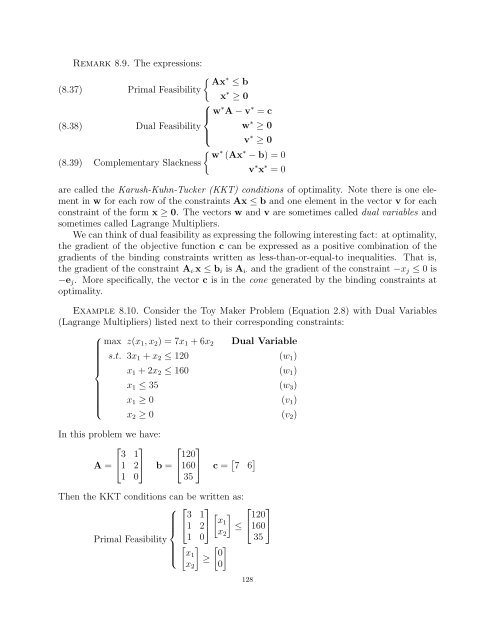
Remark 8.9. The expressions: ∗ Ax ≤ b Primal Feasibility x ∗ (8.37) ≥ 0 ⎧ ⎪⎨ w Dual Feasibility ⎪⎩ ∗ A − v ∗ = c w ∗ ≥ 0 v ∗ (8.38) ≥ 0 ∗ ∗ w (Ax − b) = 0 (8.39) Complementary Slackness v ∗ x ∗ = 0 are called the Karush-Kuhn-Tucker (KKT) conditions of optimality. Note there is one element in w for each row of the constraints Ax ≤ b and one element in the vector v for each constraint of the form x ≥ 0. The vectors w and v are sometimes called dual variables and sometimes called Lagrange Multipliers. We can think of dual feasibility as expressing the following interesting fact: at optimality, the gradient of the objective function c can be expressed as a positive combination of the gradients of the binding constraints written as less-than-or-equal-to inequalities. That is, the gradient of the constraint Ai·x ≤ bi is Ai· and the gradient of the constraint −xj ≤ 0 is −ej. More specifically, the vector c is in the cone generated by the binding constraints at optimality. Example 8.10. Consider the Toy Maker Problem (Equation 2.8) with Dual Variables (Lagrange Multipliers) listed next to their corresponding constraints: ⎧ max z(x1, x2) = 7x1 + 6x2 Dual Variable s.t. 3x1 + x2 ≤ 120 (w1) ⎪⎨ x1 + 2x2 ≤ 160 (w1) ⎪⎩ x1 ≤ 35 (w3) x1 ≥ 0 (v1) x2 ≥ 0 (v2) In this problem we have: ⎡ 3 A = ⎣1 ⎤ 1 2⎦ ⎡ b = ⎣ 1 0 120 ⎤ 160⎦ c = 35 7 6 Then the KKT conditions can be written as: ⎧ ⎡ ⎤ ⎡ 3 1 x1 ⎪⎨ ⎣1 2⎦ ≤ ⎣ x2 Primal Feasibility 1 0 ⎪⎩ 120 ⎤ 160⎦ 35 x1 0 ≥ 0 x2 128
⎧ ⎪⎨ Dual Feasibility ⎪⎩ w1 w2 w3 w1 w2 w3 v1 v2 ≥ 0 0 ⎡ 3 ⎣1 ⎤ 1 2⎦ − 1 0 v1 v2 = 7 6 ≥ 0 0 0 ⎧ ⎛⎡ ⎤ ⎪⎨ 3 1 w1 w2 w3 ⎝⎣1 2⎦ Complementary Slackness 1 0 ⎪⎩ v1 v2 x1 x2 = 0 x1 x2 ⎡ ≤ ⎣ 120 ⎤ ⎡ 160⎦ − ⎣ 35 120 ⎤⎞ 160⎦⎠ 35 Recall that at optimality, we had x1 = 16 and x2 = 72. The binding constraints in this case where 3x1 + x2 ≤ 120 x1 + 2x2 ≤ 160 To see this note that if 3(16) + 72 = 120 and 16 + 2(72) = 160. Then we should be able to express c = [7 6] (the vector of coefficients of the objective function) as a positive combination of the gradients of the binding constraints: ∇(7x1 + 6x2) = 7 6 ∇(3x1 + x2) = 3 1 ∇(x1 + 2x2) = 1 2 That is, we wish to solve the linear equation: (8.40) w1 w2 3 1 1 = 2 7 6 Note, this is how Equation 8.32 looks when we apply it to this problem. The result is a system of equations: 3w1 + w2 = 7 w1 + 2w2 = 6 A solution to this system is w1 = 8 5 and w2 = 11 5 . This fact is illustrated in Figure 8.4. Figure 8.4 shows the gradient cone formed by the binding constraints at the optimal point for the toy maker problem. Since x1, x2 > 0, we must have v1 = v2 = 0. Moreover, since x1 < 35, we know that x1 ≤ 35 is not a binding constraint and thus its dual variable w3 is also zero. This leads to the conclusion: ∗ x1 = x ∗ 2 16 72 and the KKT conditions are satisfied. ∗ w1 w∗ 2 w∗ ∗ 3 = 8/5 11/5 0 v1 v∗ 2 = 0 0 129
Page 1:
Linear Programming: Penn State Math
Page 4 and 5:
8. Caratheodory Characterization Th
Page 7 and 8:
List of Figures 1.1 Goat pen with u
Page 9 and 10:
4.6 Convex Direction: Clearly every
Page 11:
Preface Stop! Stop right now! This
Page 14 and 15:
x Goat Pen Figure 1.1. Goat pen wit
Page 16 and 17:
We have formulated the general maxi
Page 18 and 19:
Figure 1.3. Contour Plot of z = x 2
Page 20 and 21:
Figure 1.5. A Level Curve Plot with
Page 22 and 23:
and thus our vector is v = (x1 −
Page 24 and 25:
Figure 1.7. Gradients of the Bindin
Page 26 and 27:
finishing toys and 120 hours per we
Page 28 and 29:
2. Graphically Solving Linear Progr
Page 30 and 31:
S r x 0 Br( x0) Figure 2.2. A Bound
Page 32 and 33:
S Every point on this line is an al
Page 34:
6. Problems with Unbounded Feasible
Page 37:
to “prove” your example works.
Page 40 and 41:
Definition 3.6 (Matrix Transpose).
Page 42 and 43:
3. Matrices and Linear Programming
Page 44 and 45:
Remark 3.16. We can deal with const
Page 46 and 47:
Theorem 3.20. Each elementary row o
Page 48 and 49:
Gauss-Jordan Elimination Computing
Page 50 and 51:
and right hand side vector b = [7,
Page 52 and 53:
Gauss-Jordan elimination to solve t
Page 54 and 55:
which clearly has a solution for al
Page 56 and 57:
which is a contradiction. Case 2: S
Page 58 and 59:
Definition 3.46 (Basic Variables).
Page 60 and 61:
This leads to the following linear
Page 62 and 63:
This is not in a form Matlab likes,
Page 64 and 65:
Example 4.5. Figure 4.1 illustrates
Page 66 and 67:
Figure 4.3. A hyperplane in 3 dimen
Page 68 and 69:
4. Rays and Directions Recall the d
Page 70 and 71:
for all λ > 0. This can only be tr
Page 72 and 73:
Theorem 4.31. Let P ⊆ R n be a po
Page 74 and 75:
Figure 4.9. A Polyhedral Set: This
Page 76 and 77:
Figure 4.10. Visualization of the s
Page 78 and 79:
It is clear that P is bounded. In f
Page 80 and 81:
x1 x5 x2 x λx2 +(1− λ)x3 x4 x3
Page 82 and 83:
If there is some i such that c T di
Page 84 and 85:
Consider now the fact xj = 0 for al
Page 86 and 87:
Example 5.9. Consider the Toy Maker
Page 88 and 89:
using this information, we can comp
Page 90 and 91: Figure 5.1. The Simplex Algorithm:
Page 92 and 93: Using this information, we can see
Page 94 and 95: Based on this information, we can c
Page 96 and 97: Using the rule you developed in Exe
Page 98 and 99: Exercise 52. Consider the diet prob
Page 100 and 101: Suppose we choose s4 as the leaving
Page 103 and 104: CHAPTER 6 Simplex Initialization In
Page 105 and 106: A basic feasible solution for our a
Page 107 and 108: variables. This is because we start
Page 109 and 110: To remove the artificial variables
Page 111 and 112: Remark 6.6. In the case of a minimi
Page 113 and 114: Example 6.13. Suppose we solve the
Page 115 and 116: That is, s1 = −12 and s2 = −20
Page 117 and 118: The complete problem describing McL
Page 119: * data section */ data; set DAY :=
Page 122 and 123: This leads to a vector of reduced c
Page 124 and 125: 2.1. Lexicographic Minimum Ratio Te
Page 126 and 127: Proof. The initial basis Im yieds a
Page 128 and 129: for i = 1, . . . , n. Then we have:
Page 130 and 131: Revised Simplex Algorithm (1) Ident
Page 132 and 133: simplex tableau). We obtain: z1 −
Page 134 and 135: Proof. We can prove Farkas’ Lemma
Page 136 and 137: A1· Half-space cy > 0 A2· c Am·
Page 138 and 139: 3. The Karush-Kuhn-Tucker Condition
Page 142 and 143: (x ∗ 1,x ∗ 2) = (16, 72) 3x1 +
Page 144 and 145: Since w1, w2 ≥ 0, we know that w
Page 146 and 147: Example 8.13. Consider the followin
Page 148 and 149: Figure 8.5. This figure illustrates
Page 150 and 151: (9.4) Proof. Rewrite Problem D as:
Page 152 and 153: This vector will be related to c in
Page 154 and 155: 3. Strong Duality Lemma 9.7. Proble
Page 156 and 157: Likewise beginning with the KKT con
Page 158 and 159: egions are polyhedral sets 1 . Cert
Page 160 and 161: Figure 9.2. The simplex algorithm b
Page 162 and 163: If a selfish profit maximizer wishe
Page 164 and 165: Recall the optimal full tableau for
Page 166 and 167: For the sake of space, we will prov
Page 168 and 169: We can choose either s1 or s2 as a
show all

Linear Programming Lecture Notes - Penn State Personal Web Server

You also want an ePaper? Increase the reach of your titles

Delete template?

Save as template?