Linear Programming Lecture Notes - Penn State Personal Web Server

More documents

Recommendations

Info

Remark 3.16. We can deal with constraints of the form: (3.21) ai1x1 + ai2x2 + · · · + ainxn ≥ bi in a similar way. In this case we subtract a surplus variable si to obtain: ai1x1 + ai2x2 + · · · + ainxn − si = bi Again, we must have si ≥ 0. Theorem 3.17. Every linear programming problem in standard form can be put into canonical form. Proof. Recall that Ax = b if and only if Ax ≤ b and Ax ≥ b. The second inequality can be written as −Ax ≤ −b. This yields the linear programming problem: ⎧ max z(x) =c ⎪⎨ (3.22) ⎪⎩ T x s.t. Ax ≤ b − Ax ≤ −b x ≥ 0 Defining the appropriate augmented matrices allows us to convert this linear programming problem into canonical form. Exercise 24. Complete the “pedantic” proof of the preceding theorem by defining the correct augmented matrices to show that the linear program in Expression 3.22 is in canonical form. The standard solution method for linear programming models (the Simplex Algorithm) assumes that all variables are non-negative. Though this assumption can be easily relaxed, the first implementation we will study imposes this restriction. The general linear programming problem we posed in Expression 3.15 does not (necessarily) impose any sign restriction on the variables. We will show that we can transform a problem in which xi is unrestricted into a new problem in which all variables are positive. Clearly, if xi ≤ 0, then we simply replace xi by −yi in every expression and then yi ≥ 0. On the other hand, if we have the constraint xi ≥ li, then clearly we can write yi = xi − li and yi ≥ 0. We can then replace xi by yi + li in every equation or inequality where xi appears. Finally, if xi ≤ ui, but xi may be negative, then we may write yi = ui − xi. Clearly, yi ≥ 0 and we can replace xi by ui − yi in every equation or inequality where xi appears. If xi is unrestricted in sign and has no upper or lower bounds, then let xi = yi − zi where yi, zi ≥ 0 and replace xi by (yi − zi) in the objective, equations and inequalities of a general linear programming problem. Since yi, zi ≥ 0 and may be given any values as a part of the solution, clearly xi may take any value in R. Exercise 25. Convince yourself that the general linear programming problem shown in Expression 3.15 can be converted into canonical (or standard) form using the following steps: (1) Every constraint of the form xi ≤ ui can be dealt with by substituting yi = ui − xi, yi ≥ 0. (2) Every constraint of the form li ≤ xi can be dealt with by substituting yi = xi − li, yi ≥ 0. 32
(3) If xi is unrestricted in any way, then we can variables yi and zi so that xi = yi − zi where yi, zi ≥ 0. (4) Any equality constraints Hx = r can be transformed into inequality constraints. Thus, Expression 3.15 can be transformed to standard form. [Hint: No hint, the hint is in the problem.] 4. Gauss-Jordan Elimination and Solution to <strong>Linear</strong> Equations In this sub-section, we’ll review Gauss-Jordan Elimination as a solution method for linear equations. We’ll use Gauss-Jordan Elimination extensively in the coming chapters. Definition 3.18 (Elementary Row Operation). Let A ∈ R m×n be a matrix. Recall Ai· is the i th row of A. There are three elementary row operations: (1) (Scalar Multiplication of a Row) Row Ai· is replaced by αAi·, where α ∈ R and α = 0. (2) (Row Swap) Row Ai· is swapped with Row Aj· for i = j. (3) (Scalar Multiplication and Addition) Row Aj· is replaced by αAi· + Aj· for α ∈ R and i = j. 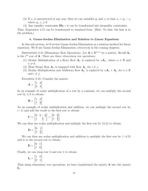Example 3.19. Consider the matrix: 1 2 A = 3 4 In an example of scalar multiplication of a row by a constant, we can multiply the second row by 1/3 to obtain: 1 2 B = 1 4 3 As an example of scalar multiplication and addition, we can multiply the second row by (−1) and add the result to the first row to obtain: 4 2 0 2 − 0 C = 3 4 = 3 1 1 3 4 3 We can then use scalar multiplication and multiply the first row by (3/2) to obtain: 0 1 D = 1 4 3 We can then use scalar multiplication and addition to multiply the first row by (−4/3) add it to the second row to obtain: 0 1 E = 1 0 Finally, we can swap row 2 and row 1 to obtain: 1 0 I2 = 0 1 Thus using elementary row operations, we have transformed the matrix A into the matrix I2. 33
Page 1: Linear Programming: Penn State Math
Page 4 and 5: 8. Caratheodory Characterization Th
Page 7 and 8: List of Figures 1.1 Goat pen with u
Page 9 and 10: 4.6 Convex Direction: Clearly every
Page 11: Preface Stop! Stop right now! This
Page 14 and 15: x Goat Pen Figure 1.1. Goat pen wit
Page 16 and 17: We have formulated the general maxi
Page 18 and 19: Figure 1.3. Contour Plot of z = x 2
Page 20 and 21: Figure 1.5. A Level Curve Plot with
Page 22 and 23: and thus our vector is v = (x1 −
Page 24 and 25: Figure 1.7. Gradients of the Bindin
Page 26 and 27: finishing toys and 120 hours per we
Page 28 and 29: 2. Graphically Solving Linear Progr
Page 30 and 31: S r x 0 Br( x0) Figure 2.2. A Bound
Page 32 and 33: S Every point on this line is an al
Page 34: 6. Problems with Unbounded Feasible
Page 37: to “prove” your example works.
Page 40 and 41: Definition 3.6 (Matrix Transpose).
Page 42 and 43: 3. Matrices and Linear Programming
Page 46 and 47: Theorem 3.20. Each elementary row o
Page 48 and 49: Gauss-Jordan Elimination Computing
Page 50 and 51: and right hand side vector b = [7,
Page 52 and 53: Gauss-Jordan elimination to solve t
Page 54 and 55: which clearly has a solution for al
Page 56 and 57: which is a contradiction. Case 2: S
Page 58 and 59: Definition 3.46 (Basic Variables).
Page 60 and 61: This leads to the following linear
Page 62 and 63: This is not in a form Matlab likes,
Page 64 and 65: Example 4.5. Figure 4.1 illustrates
Page 66 and 67: Figure 4.3. A hyperplane in 3 dimen
Page 68 and 69: 4. Rays and Directions Recall the d
Page 70 and 71: for all λ > 0. This can only be tr
Page 72 and 73: Theorem 4.31. Let P ⊆ R n be a po
Page 74 and 75: Figure 4.9. A Polyhedral Set: This
Page 76 and 77: Figure 4.10. Visualization of the s
Page 78 and 79: It is clear that P is bounded. In f
Page 80 and 81: x1 x5 x2 x λx2 +(1− λ)x3 x4 x3
Page 82 and 83: If there is some i such that c T di
Page 84 and 85: Consider now the fact xj = 0 for al
Page 86 and 87: Example 5.9. Consider the Toy Maker
Page 88 and 89: using this information, we can comp
Page 90 and 91: Figure 5.1. The Simplex Algorithm:
Page 92 and 93: Using this information, we can see
Page 94 and 95:
Based on this information, we can c
Page 96 and 97:
Using the rule you developed in Exe
Page 98 and 99:
Exercise 52. Consider the diet prob
Page 100 and 101:
Suppose we choose s4 as the leaving
Page 103 and 104:
CHAPTER 6 Simplex Initialization In
Page 105 and 106:
A basic feasible solution for our a
Page 107 and 108:
variables. This is because we start
Page 109 and 110:
To remove the artificial variables
Page 111 and 112:
Remark 6.6. In the case of a minimi
Page 113 and 114:
Example 6.13. Suppose we solve the
Page 115 and 116:
That is, s1 = −12 and s2 = −20
Page 117 and 118:
The complete problem describing McL
Page 119:
* data section */ data; set DAY :=
Page 122 and 123:
This leads to a vector of reduced c
Page 124 and 125:
2.1. Lexicographic Minimum Ratio Te
Page 126 and 127:
Proof. The initial basis Im yieds a
Page 128 and 129:
for i = 1, . . . , n. Then we have:
Page 130 and 131:
Revised Simplex Algorithm (1) Ident
Page 132 and 133:
simplex tableau). We obtain: z1 −
Page 134 and 135:
Proof. We can prove Farkas’ Lemma
Page 136 and 137:
A1· Half-space cy > 0 A2· c Am·
Page 138 and 139:
3. The Karush-Kuhn-Tucker Condition
Page 140 and 141:
Remark 8.9. The expressions: ∗ A
Page 142 and 143:
(x ∗ 1,x ∗ 2) = (16, 72) 3x1 +
Page 144 and 145:
Since w1, w2 ≥ 0, we know that w
Page 146 and 147:
Example 8.13. Consider the followin
Page 148 and 149:
Figure 8.5. This figure illustrates
Page 150 and 151:
(9.4) Proof. Rewrite Problem D as:
Page 152 and 153:
This vector will be related to c in
Page 154 and 155:
3. Strong Duality Lemma 9.7. Proble
Page 156 and 157:
Likewise beginning with the KKT con
Page 158 and 159:
egions are polyhedral sets 1 . Cert
Page 160 and 161:
Figure 9.2. The simplex algorithm b
Page 162 and 163:
If a selfish profit maximizer wishe
Page 164 and 165:
Recall the optimal full tableau for
Page 166 and 167:
For the sake of space, we will prov
Page 168 and 169:
We can choose either s1 or s2 as a
show all

Linear Programming Lecture Notes - Penn State Personal Web Server

Create successful ePaper yourself

Delete template?

Save as template?