Linear Programming Lecture Notes - Penn State Personal Web Server

More documents

Recommendations

Info

which is a contradiction. Case 2: Suppose that the size of the largest set of linearly independent rows is k. Denote such a set by S = {as1, . . . , ask }. There are several possibilities: (i) Both ai and aj are in this set. In this case, we simply replace our argument above with constants α1 through αk and the result is the same. (ii) ai and aj are not in this set, in which case we know that there are αs1, . . . , αsk and βs1, . . . , βsk so that: αs1a1 + · · · + αsk ak = ai βs1a1 + · · · + βsk ak = aj But this implies that αai + aj can also be written as a linear combination of the elements of S and thus the rank of A ′ is no larger than the rank of A. (iii) Now suppose that ai in the set S. Then there are constants αs1, . . . , αsk αs1a1 + · · · + αsk ak = aj Without loss of generality, suppose that ai = as1 then: αai + αs1ai + αs2as2 + · · · + αsk ak = αai + aj so that: Again, this implies that αai + aj is still a linear combination of the elements of S and so we cannot have increased the size of the largest linearly independent set of vectors, nor could we have decreased it. (iv) Finally, suppose that aj ∈ S. Again let aj = as1. Then there are constants αs1, . . . , αsk αs1aJ + αs2as2 + · · · + αskask = ai Apply Lemma 3.38 to replace aj in S with some other row vector al. If l = i, then we reduce to sub-case (iii). If l = i, then we reduce to sub-case (ii). Finally, suppose we multiply a row by α. This is reduces to the case of multiplying row i by α − 1 and adding it to row i, which is covered in the above analysis. This completes the proof. We have the following theorem, whose proof is again outside the scope of this course. There are very nice proofs available in [Lan87]. Theorem 3.42. If A ∈ R m×n is a matrix, then the row rank of A is equal to the column rank of A. Further, rank(A) ≤ min{m, n}. Lastly, we will not prove the following theorem, but it should be clear from all the work we have done up to this point. Theorem 3.43. If A ∈ R m×m (i.e., A is a square matrix) and rank(A) = m, then A is invertible. Definition 3.44. Suppose that A ∈ R m×n and let m ≤ n. Then A has full row rank if rank(A) = m. 44
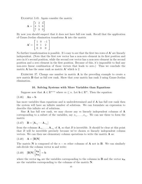
Example 3.45. Again consider the matrix ⎡ ⎤ 1 2 3 A = ⎣4 5 6⎦ 7 8 9 By now you should suspect that it does not have full row rank. Recall that the application of Gauss-Jordan elimination transforms A into the matrix A ′ ⎡ ⎤ 1 0 −1 = ⎣ 0 1 2 ⎦ 0 0 0 No further transformation is possible. It’s easy to see that the first two rows of A ′ are linearly independent. (Note that the first row vector has a non-zero element in its first position and zero in it’s second position, while the second row vector has a non-zero element in the second position and a zero element in the first position. Because of this, it’s impossible to find any non-zero linear combination of those vectors that leads to zero.) Thus we conclude the matrix A has the same rank as matrix A ′ which is 2. Exercise 37. Change one number in matrix A in the preceding example to create a new matrix B that as full row rank. Show that your matrix has rank 3 using Gauss-Jordan elimination. 10. Solving Systems with More Variables than Equations Suppose now that A ∈ R m×n where m ≤ n. Let b ∈ R m . Then the equation: (3.46) Ax = b has more variables than equations and is underdetermined and if A has full row rank then the system will have an infinite number of solutions. We can formulate an expression to describe this infinite set of solutions. Sine A has full row rank, we may choose any m linearly independent columns of A corresponding to a subset of the variables, say xi1, . . . , xim. We can use these to form the matrix (3.47) B = [A·i1 · · · A·im] from the columns A·i1, . . . , A·im of A, so that B is invertible. It should be clear at this point that B will be invertible precisely because we’ve chosen m linearly independent column vectors. We can then use elementary column operations to write the matrix A as: (3.48) A = [B|N] The matrix N is composed of the n − m other columns of A not in B. We can similarly sub-divide the column vector x and write: xB (3.49) [B|N] = b xN where the vector xB are the variables corresponding to the columns in B and the vector xN are the variables corresponding to the columns of the matrix N. 45
Page 1:
Linear Programming: Penn State Math
Page 4 and 5:
8. Caratheodory Characterization Th
Page 7 and 8: List of Figures 1.1 Goat pen with u
Page 9 and 10: 4.6 Convex Direction: Clearly every
Page 11: Preface Stop! Stop right now! This
Page 14 and 15: x Goat Pen Figure 1.1. Goat pen wit
Page 16 and 17: We have formulated the general maxi
Page 18 and 19: Figure 1.3. Contour Plot of z = x 2
Page 20 and 21: Figure 1.5. A Level Curve Plot with
Page 22 and 23: and thus our vector is v = (x1 −
Page 24 and 25: Figure 1.7. Gradients of the Bindin
Page 26 and 27: finishing toys and 120 hours per we
Page 28 and 29: 2. Graphically Solving Linear Progr
Page 30 and 31: S r x 0 Br( x0) Figure 2.2. A Bound
Page 32 and 33: S Every point on this line is an al
Page 34: 6. Problems with Unbounded Feasible
Page 37: to “prove” your example works.
Page 40 and 41: Definition 3.6 (Matrix Transpose).
Page 42 and 43: 3. Matrices and Linear Programming
Page 44 and 45: Remark 3.16. We can deal with const
Page 46 and 47: Theorem 3.20. Each elementary row o
Page 48 and 49: Gauss-Jordan Elimination Computing
Page 50 and 51: and right hand side vector b = [7,
Page 52 and 53: Gauss-Jordan elimination to solve t
Page 54 and 55: which clearly has a solution for al
Page 58 and 59: Definition 3.46 (Basic Variables).
Page 60 and 61: This leads to the following linear
Page 62 and 63: This is not in a form Matlab likes,
Page 64 and 65: Example 4.5. Figure 4.1 illustrates
Page 66 and 67: Figure 4.3. A hyperplane in 3 dimen
Page 68 and 69: 4. Rays and Directions Recall the d
Page 70 and 71: for all λ > 0. This can only be tr
Page 72 and 73: Theorem 4.31. Let P ⊆ R n be a po
Page 74 and 75: Figure 4.9. A Polyhedral Set: This
Page 76 and 77: Figure 4.10. Visualization of the s
Page 78 and 79: It is clear that P is bounded. In f
Page 80 and 81: x1 x5 x2 x λx2 +(1− λ)x3 x4 x3
Page 82 and 83: If there is some i such that c T di
Page 84 and 85: Consider now the fact xj = 0 for al
Page 86 and 87: Example 5.9. Consider the Toy Maker
Page 88 and 89: using this information, we can comp
Page 90 and 91: Figure 5.1. The Simplex Algorithm:
Page 92 and 93: Using this information, we can see
Page 94 and 95: Based on this information, we can c
Page 96 and 97: Using the rule you developed in Exe
Page 98 and 99: Exercise 52. Consider the diet prob
Page 100 and 101: Suppose we choose s4 as the leaving
Page 103 and 104: CHAPTER 6 Simplex Initialization In
Page 105 and 106: A basic feasible solution for our a
Page 107 and 108:
variables. This is because we start
Page 109 and 110:
To remove the artificial variables
Page 111 and 112:
Remark 6.6. In the case of a minimi
Page 113 and 114:
Example 6.13. Suppose we solve the
Page 115 and 116:
That is, s1 = −12 and s2 = −20
Page 117 and 118:
The complete problem describing McL
Page 119:
* data section */ data; set DAY :=
Page 122 and 123:
This leads to a vector of reduced c
Page 124 and 125:
2.1. Lexicographic Minimum Ratio Te
Page 126 and 127:
Proof. The initial basis Im yieds a
Page 128 and 129:
for i = 1, . . . , n. Then we have:
Page 130 and 131:
Revised Simplex Algorithm (1) Ident
Page 132 and 133:
simplex tableau). We obtain: z1 −
Page 134 and 135:
Proof. We can prove Farkas’ Lemma
Page 136 and 137:
A1· Half-space cy > 0 A2· c Am·
Page 138 and 139:
3. The Karush-Kuhn-Tucker Condition
Page 140 and 141:
Remark 8.9. The expressions: ∗ A
Page 142 and 143:
(x ∗ 1,x ∗ 2) = (16, 72) 3x1 +
Page 144 and 145:
Since w1, w2 ≥ 0, we know that w
Page 146 and 147:
Example 8.13. Consider the followin
Page 148 and 149:
Figure 8.5. This figure illustrates
Page 150 and 151:
(9.4) Proof. Rewrite Problem D as:
Page 152 and 153:
This vector will be related to c in
Page 154 and 155:
3. Strong Duality Lemma 9.7. Proble
Page 156 and 157:
Likewise beginning with the KKT con
Page 158 and 159:
egions are polyhedral sets 1 . Cert
Page 160 and 161:
Figure 9.2. The simplex algorithm b
Page 162 and 163:
If a selfish profit maximizer wishe
Page 164 and 165:
Recall the optimal full tableau for
Page 166 and 167:
For the sake of space, we will prov
Page 168 and 169:
We can choose either s1 or s2 as a
show all

Linear Programming Lecture Notes - Penn State Personal Web Server

You also want an ePaper? Increase the reach of your titles

Delete template?

Save as template?