Linear Programming Lecture Notes - Penn State Personal Web Server

More documents

Recommendations

Info

At this point, we have eliminated both artificial variables from the basis and we have identified and initial basic feasible solution to the original problem: x1 = 4, x2 = 4, s1 = 0 and s2 = 0. The process of moving to a feasible solution in the original problem is shown in Figure 6.1. Figure 6.1. Finding an initial feasible point: Artificial variables are introduced into the problem. These variables allow us to move through non-feasible space. Once we reach a feasible extreme point, the process of optimizing Problem P1 stops. We could now continue on to solve the initial problem we were given. At this point, our basic feasible solution makes x2 and x1 basic variables and s1 and s2 non-basic variables. Our problem data are: x2 xB = x1 s1 xN = s2 Note that we keep the basic variables in the order in which we find them at the end of the solution to our first problem. 1 2 −1 0 12 A = b = 2 3 0 −1 20 B = cB = 2 1 3 2 2 1 N = cN = −1 0 0 −1 0 0 B −1 b = c T BB −1 b = 12 c T BB −1 N − c T N = −1 0 Notice that we don’t have to do a lot of work to get this information out of the last tableau in Expression 6.11. The matrix B −1 is actually positioned in the columns below the artificial 94 4 4
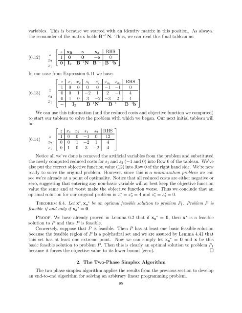
variables. This is because we started with an identity matrix in this position. As always, the remainder of the matrix holds B −1 N. Thus, we can read this final tableau as: (6.12) z x2 x1 ⎡ ⎣ z xB s xa RHS 1 0 0 −e 0 0 I2 B −1 N B −1 B −1 b In our case from Expression 6.11 we have: ⎡ (6.13) z x2 x1 ⎢ ⎣ z x1 x2 s1 s2 xa1 xa2 RHS 1 0 0 0 0 −1 −1 0 0 0 1 −2 1 2 −1 4 0 1 0 3 −2 −3 2 4 − I2 B −1 N B −1 B −1 b ⎤ ⎦ We can use this information (and the reduced costs and objective function we computed) to start our tableau to solve the problem with which we began. Our next initial tableau will be: (6.14) z x2 x1 ⎡ ⎢ ⎣ z x1 x2 s1 s2 RHS 1 0 0 −1 0 12 0 0 1 −2 1 4 0 1 0 3 −2 4 ⎤ ⎥ ⎦ Notice all we’ve done is removed the artificial variables from the problem and substituted the newly computed reduced costs for s1 and s2 (−1 and 0) into Row 0 of the tableau. We’ve also put the correct objective function value (12) into Row 0 of the right hand side. We’re now ready to solve the original problem. However, since this is a minimization problem we can see we’re already at a point of optimality. Notice that all reduced costs are either negative or zero, suggesting that entering any non-basic variable will at best keep the objective function value the same and at worst make the objective function worse. Thus we conclude that an optimal solution for our original problem is x ∗ 1 = x ∗ 2 = 4 and s ∗ 1 = s ∗ 2 = 0. Theorem 6.4. Let x ∗ , xa ∗ be an optimal feasible solution to problem P1. Problem P is feasible if and only if xa ∗ = 0. Proof. We have already proved in Lemma 6.2 that if xa ∗ = 0, then x ∗ is a feasible solution to P and thus P is feasible. Conversely, suppose that P is feasible. Then P has at least one basic feasible solution because the feasible region of P is a polyhedral set and we are assured by Lemma 4.41 that this set has at least one extreme point. Now we can simply let xa ∗ = 0 and x be this basic feasible solution to problem P . Then this is clearly an optimal solution to problem P1 because it forces the objective value to its lower bound (zero). ⎤ ⎥ ⎦ 2. The Two-Phase Simplex Algorithm The two phase simplex algorithm applies the results from the previous section to develop an end-to-end algorithm for solving an arbitrary linear programming problem. 95
Page 1:
Linear Programming: Penn State Math
Page 4 and 5:
8. Caratheodory Characterization Th
Page 7 and 8:
List of Figures 1.1 Goat pen with u
Page 9 and 10:
4.6 Convex Direction: Clearly every
Page 11:
Preface Stop! Stop right now! This
Page 14 and 15:
x Goat Pen Figure 1.1. Goat pen wit
Page 16 and 17:
We have formulated the general maxi
Page 18 and 19:
Figure 1.3. Contour Plot of z = x 2
Page 20 and 21:
Figure 1.5. A Level Curve Plot with
Page 22 and 23:
and thus our vector is v = (x1 −
Page 24 and 25:
Figure 1.7. Gradients of the Bindin
Page 26 and 27:
finishing toys and 120 hours per we
Page 28 and 29:
2. Graphically Solving Linear Progr
Page 30 and 31:
S r x 0 Br( x0) Figure 2.2. A Bound
Page 32 and 33:
S Every point on this line is an al
Page 34:
6. Problems with Unbounded Feasible
Page 37:
to “prove” your example works.
Page 40 and 41:
Definition 3.6 (Matrix Transpose).
Page 42 and 43:
3. Matrices and Linear Programming
Page 44 and 45:
Remark 3.16. We can deal with const
Page 46 and 47:
Theorem 3.20. Each elementary row o
Page 48 and 49:
Gauss-Jordan Elimination Computing
Page 50 and 51:
and right hand side vector b = [7,
Page 52 and 53:
Gauss-Jordan elimination to solve t
Page 54 and 55:
which clearly has a solution for al
Page 56 and 57: which is a contradiction. Case 2: S
Page 58 and 59: Definition 3.46 (Basic Variables).
Page 60 and 61: This leads to the following linear
Page 62 and 63: This is not in a form Matlab likes,
Page 64 and 65: Example 4.5. Figure 4.1 illustrates
Page 66 and 67: Figure 4.3. A hyperplane in 3 dimen
Page 68 and 69: 4. Rays and Directions Recall the d
Page 70 and 71: for all λ > 0. This can only be tr
Page 72 and 73: Theorem 4.31. Let P ⊆ R n be a po
Page 74 and 75: Figure 4.9. A Polyhedral Set: This
Page 76 and 77: Figure 4.10. Visualization of the s
Page 78 and 79: It is clear that P is bounded. In f
Page 80 and 81: x1 x5 x2 x λx2 +(1− λ)x3 x4 x3
Page 82 and 83: If there is some i such that c T di
Page 84 and 85: Consider now the fact xj = 0 for al
Page 86 and 87: Example 5.9. Consider the Toy Maker
Page 88 and 89: using this information, we can comp
Page 90 and 91: Figure 5.1. The Simplex Algorithm:
Page 92 and 93: Using this information, we can see
Page 94 and 95: Based on this information, we can c
Page 96 and 97: Using the rule you developed in Exe
Page 98 and 99: Exercise 52. Consider the diet prob
Page 100 and 101: Suppose we choose s4 as the leaving
Page 103 and 104: CHAPTER 6 Simplex Initialization In
Page 105: A basic feasible solution for our a
Page 109 and 110: To remove the artificial variables
Page 111 and 112: Remark 6.6. In the case of a minimi
Page 113 and 114: Example 6.13. Suppose we solve the
Page 115 and 116: That is, s1 = −12 and s2 = −20
Page 117 and 118: The complete problem describing McL
Page 119: * data section */ data; set DAY :=
Page 122 and 123: This leads to a vector of reduced c
Page 124 and 125: 2.1. Lexicographic Minimum Ratio Te
Page 126 and 127: Proof. The initial basis Im yieds a
Page 128 and 129: for i = 1, . . . , n. Then we have:
Page 130 and 131: Revised Simplex Algorithm (1) Ident
Page 132 and 133: simplex tableau). We obtain: z1 −
Page 134 and 135: Proof. We can prove Farkas’ Lemma
Page 136 and 137: A1· Half-space cy > 0 A2· c Am·
Page 138 and 139: 3. The Karush-Kuhn-Tucker Condition
Page 140 and 141: Remark 8.9. The expressions: ∗ A
Page 142 and 143: (x ∗ 1,x ∗ 2) = (16, 72) 3x1 +
Page 144 and 145: Since w1, w2 ≥ 0, we know that w
Page 146 and 147: Example 8.13. Consider the followin
Page 148 and 149: Figure 8.5. This figure illustrates
Page 150 and 151: (9.4) Proof. Rewrite Problem D as:
Page 152 and 153: This vector will be related to c in
Page 154 and 155: 3. Strong Duality Lemma 9.7. Proble
Page 156 and 157:
Likewise beginning with the KKT con
Page 158 and 159:
egions are polyhedral sets 1 . Cert
Page 160 and 161:
Figure 9.2. The simplex algorithm b
Page 162 and 163:
If a selfish profit maximizer wishe
Page 164 and 165:
Recall the optimal full tableau for
Page 166 and 167:
For the sake of space, we will prov
Page 168 and 169:
We can choose either s1 or s2 as a
show all

Linear Programming Lecture Notes - Penn State Personal Web Server

Create successful ePaper yourself

Delete template?

Save as template?