Linear Programming Lecture Notes - Penn State Personal Web Server

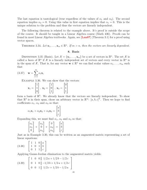
The last equation is tautological (true regardless of the values of α1 and α2). The second
equation implies α2 = 0. Using this value in first equation implies that α1 = 0. This is the
unique solution to the problem and thus the vectors are linearly independent.
The following theorem is related to the example above. It’s proof is outside the scope
of the course. It should be taught in a Linear Algebra course (Math 436). Proofs can be
found in most Linear Algebra textbooks. Again, see [Lan87] (Theorem 3.1) for a proof using
vector spaces.
Theorem 3.34. Let x1, . . . , xm ∈ R n . If m > n, then the vectors are linearly dependent.
8. Basis
Definition 3.35 (Basis). Let X = {x1, . . . , xm} be a set of vectors in Rn . The set X is
called a basis of Rn if X is a linearly independent set of vectors and every vector in Rn is
in the span of X . That is, for any vector w ∈ Rn we can find scalar values α1, . . . , αm such
that
m
(3.37) w =
i=1
αixi
Example 3.36. We can show that the vectors:
⎡
x1 = ⎣ 1
⎤ ⎡
1⎦
, x2 = ⎣
0
1
⎤ ⎡
0⎦
, x3 = ⎣
1
0
⎤
1⎦
1
form a basis of R 3 . We already know that the vectors are linearly independent. To show
that R 3 is in their span, chose an arbitrary vector in R m : [a, b, c] T . Then we hope to find
coefficients α1, α2 and α3 so that:
⎡
α1x1 + α2x2 + α3x3 = ⎣ a
⎤
b⎦
c
Expanding this, we must find α1, α2 and α3 so that:
⎡
⎣ α1
⎤ ⎡
α1⎦
+ ⎣
0
α2
⎤ ⎡
0 ⎦ + ⎣ 0
⎤ ⎡
α3⎦
= ⎣ a
⎤
b⎦
c
α2
α3
Just as in Example 3.30, this can be written as an augmented matrix representing a set of
linear equations:
⎡
1 1 0
(3.38) ⎣ 1 0 1
⎤
a
b ⎦
0 1 1 c
Applying Gauss-Jordan elimination to the augmented matrix yields:
⎡
⎤
1 0 0 1/2 a + 1/2 b − 1/2 c
(3.39)
⎢
⎣ 0 1 0
⎥
−1/2 b + 1/2 a + 1/2 c ⎦
0 0 1 1/2 c + 1/2 b − 1/2 a
41